Download
1 / 33
330 likes | 459 Views
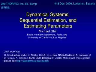
4–8 Dec. 2006, Landshut, Bavaria. 2nd THORPEX Intl. Sci. Symp. (STISS). Dynamical Systems, Sequential Estimation, and Estimating Parameters. Michael Ghil Ecole Normale Supérieure, Paris, and University of California, Los Angeles. Joint work with

E N D
4–8 Dec. 2006, Landshut, Bavaria 2nd THORPEX Intl. Sci. Symp. (STISS) Dynamical Systems, Sequential Estimation, and Estimating Parameters Michael Ghil Ecole Normale Supérieure, Paris, and University of California, Los Angeles Joint work with D. Kondrashov and J. D. Neelin, UCLA; C.-J. Sun, NASA Goddard; A. Carrassi, U. of Ferrara; A. Trevisan, ISAC-CNR, Bologna; F. Uboldi, Milano; and many others: please see http://www.atmos.ucla.edu/tcd/
Outline • Data in meteorology and oceanography - in situ & remotely sensed • Basic ideas, data types, & issues • how to combine data with models • transfer of information - between variables & regions • stability of the fcst.–assimilation cycle • filters & smoothers • Parameter estimation - model parameters - noise parameters – at & below grid scale • Subgrid-scale parameterizations - deterministic (“classic”) - stochastic – “dynamics” & “physics” • Novel areas of application - space physics - shock waves in solids - macroeconomics • Concluding remarks
Main issues • The solid earth stays put to be observed, the atmosphere, the oceans, & many other things, do not. • Two types of information: - direct observations, and - indirect dynamics (from past observations); both have errors. • Combinethe two in (an) optimal way(s) • Advanced data assimilation methods provide such ways: - sequential estimation the Kalman filter(s), and - control theory the adjoint method(s) • The two types of methods are essentially equivalent for simple linear systems (the duality principle)
Main issues (continued) • Their performance differs for large nonlinear systems in: - accuracy, and - computational efficiency • Study optimal combination(s), as well as improvements over currently operational methods (OI, 4-D Var, PSAS, EnKF).
Space physics data Space platforms in Earth’s magnetosphere
Basic concepts: barotropic model Shallow-water equations in 1-D, linearized about (U,0,), fU = – y U = 20 ms–1, f = 10–4s–1, = gH, H 3 km. PDE system discretized by finite differences, periodic B. C. Hk: observations at synoptic times, over land only. Ghil et al. (1981), Cohn & Dee (Ph.D. theses, 1982 & 1983), etc.
Conventional network Relative weight of observational vs. model errors P∞ = QR/[Q + (1 – 2)R] (a) Q = 0 P∞ = 0 (b) Q ≠ 0 (i), (ii) and (iii): • “good” observations R << Q P∞ ≈ R; (ii)“poor” observations R >> QP∞ ≈ Q/(1 – 2); (iii) always (provided 2 < 1) P∞ ≤ min {R, Q/(1 – 2)}.
{6h fcst} - {conventional (NoSat)} Advection of information b) {“first guess”} - {FGGE analysis} Upper panel (NoSat): Errors advected off the ocean 300 {“first guess”} - {FGGE analysis} Lower panel (Sat): Errors drastically reduced, as info. now comes in, off the ocean 300 Halem, Kalnay, Baker & Atlas (BAMS, 1982)
Outline • Data in meteorology and oceanography - in situ & remotely sensed Basic ideas, data types, & issues • how to combine data with models • stability of the fcst.–assimilation cycle • filters & smoothers • Parameter estimation - model parameters - noise parameters – at & below grid scale • Subgrid-scale parameterizations - deterministic (“classic”) - stochastic – “dynamics” & “physics” • Novel areas of application - space physics - shock waves in solids - macroeconomics • Concluding remarks
Error components inforecast–analysis cycle The relative contributions to error growth of • analysis error • intrinsic error growth • modeling error (stochastic?)
Assimilation of observations: Stability considerations Free-System Dynamics(sequential-discrete formulation): Standard breeding forecast state; model integration from a previous analysis Corresponding perturbative (tangent linear) equation Observationally Forced System Dynamics(sequential-discrete formulation): BDAS If observations are available and we assimilate them: Evolutive equation of the system, subject to forcing by the assimilated data Corresponding perturbative (tangent linear) equation, if the same observations are assimilated in the perturbed trajectories as in the control solution • The matrix (I – KH) is expected, in general, to have a stabilizing effect; • the free-system instabilities, which dominate the forecast step error growth, can be reduced during the analysis step. Joint work with A. Carrassi, A. Trevisan & F. Uboldi
Stabilization of the forecast–assimilation system – I Assimilation experiment with a low-order chaotic model - Periodic 40-variable Lorenz (1996) model; - Assimilation algorithms: replacement (Trevisan & Uboldi, 2004), replacement + one adaptive obs’n located by multiple replication (Lorenz, 1996), replacement + one adaptive obs’n located by BDAS and assimilated by AUS (Trevisan & Uboldi, 2004). BDAS: Breeding on the Data Assimilation System AUS: Assimilation in the Unstable Subspace Trevisan & Uboldi (JAS, 2004)
Stabilization of the forecast–assimilation system – II Assimilation experiment with the 40-variable Lorenz (1996) model Spectrum of Lyapunov exponents: Red: free system Dark blue: AUS with 3-hr updates Purple: AUS with 2-hr updates Light blue: AUS with 1-hr updates Carrassi, Ghil, Trevisan & Uboldi, 2006, submitted
Stabilization of the forecast–assimilation system – III Assimilation experiment with an intermediate atmospheric circulation model - 64-longitudinal x 32-latitudinal x 5 levels periodic channel QG-model (Rotunno & Bao, 1996) - Perfect-model assumption - Assimilation algorithms: 3-DVar (Morss, 2001); AUS (Uboldi et al., 2005; Carrassi et al., 2006) Observational forcing Unstable subspace reduction Free System Leading exponent: max ≈ 0.31 days–1; Doubling time ≈ 2.2 days; Number of positive exponents: N+ = 24; Kaplan-Yorke dimension ≈ 65.02. 3-DVar–BDAS Leading exponent: max ≈ 6x10⁻³ days–1; AUS–BDAS Leading exponent: max ≈ – 0.52x10⁻³ days–1
Outline • Data in meteorology and oceanography - in situ & remotely sensed • Basic ideas, data types, & issues • how to combine data with models • filters & smoothers - stability of the fcst.-assimilation cycle Parameter estimation - model parameters - noise parameters – at & below grid scale • Subgrid-scale parameterizations - deterministic (“classic”) - stochastic – “dynamics” & “physics” • Novel areas of application - space physics - shock waves in solids - macroeconomics • Concluding remarks
Estimating noise – I 1 Q1 = Qslow , Q2 = Qfast , Q3 =0; R1 = 0, R2 = 0, R3 =R; Q = ∑ iQi; R = ∑ iRi ; (0) = (6.0, 4.0, 4.5)T; Q(0) = 25*I. Dee et al. (1985, IEEE Trans.Autom. Control, AC-30) estimated 2 true ( =1) 3 Poor convergence for Qfast?
Estimating noise – II 1 Same choice of (0), Qi , and Ribut 1 0.8 0 (0) = 25 *0.8 1 0 0 0 1 Dee et al. (1985, IEEE Trans.Autom. Control, AC-30) 2 estimated true ( = 1) 3 Good convergence for Qfast!
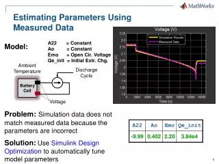
Sequential parameter estimation • “State augmentation” method – uncertain parameters are treated as additional state variables. • Example: one unknown parameter • The parameters are not directly observable, butthe cross-covariances drive parameter changes from innovations of the state: • Parameter estimation is always a nonlinear problem, even if the model is linear in terms of the model state: use Extended Kalman Filter (EKF).
Parameter estimation for coupled O-A system Forecast using wrong Forecast using wrong and s • Intermediate coupled model (ICM: Jin & Neelin, JAS, 1993) • Estimate the state vector W = (T’, h, u, v), along with the coupling parameter and surface-layer coefficient s by assimilating data from a single meridional section. • The ICM model has errors in its initial state, in the wind stress forcing & in the parameters. • M. Ghil (1997, JMSJ); Hao & Ghil (1995, Proc. WMO Symp. DA Tokyo); Sun et al. (2002, MWR). • Current work with D. Kondrashov, J.D. Neelin, & C.-j. Sun. Reference solution Assimilation result Reference solution Assimilation result
Convergence of Parameter Values – I Identical-twin experiments
Convergence of Parameter Values – II Real SSTA data
Computational advances a) Hardware - more computing power (CPU throughput) - larger & faster memory (3-tier) b) Software -better numerical implementations of algorithms - automatic adjoints - block-banded, reduced-rank & other sparse-matrix algorithms - better ensemble filters - efficient parallelization, …. How much DA vs. forecast? - Design integrated observing–forecast–assimilation systems!
Observing system design Need no more (independent) observations than d-o-f to be tracked: - “features” (Ide & Ghil, 1997a, b, DAO); - instabilities (Todling & Ghil, 1994 + Ghil & Todling, 1996, MWR); - trade-off between mass & velocity field (Jiang & Ghil, JPO, 1993). The cost of advanced DA is muchless than that of instruments & platforms: - at best use DA instead of instruments & platforms. - at worst use DA to determine which instruments & platforms (advancedOSSE) Use any observations, if forward modeling is possible (observing operator H) -satellite images, 4-D observations; - pattern recognition in observations and in phase-space statistics.
Conclusion • No observing system without data assimilation and no assimilation without dynamicsa • Quote of the day: “You cannot step into the same riverb twicec” (Heracleitus, Trans. Basil. Phil. Soc. Miletus, cca. 500 B.C.) aof state and errors bMeandros c “You cannot do so even once” (subsequent development of “flux” theory by Plato, cca. 400 B.C.) =Everything flows
Evolution of DA – I Transition from “early”to “mature” phase of DA in NWP: • no Kalman filter(Ghil et al., 1981(*)) • no adjoint(Lewis & Derber, Tellus, 1985); Le Dimet & Talagrand (Tellus, 1986) (*) Bengtsson, Ghil & Källén (Eds., 1981), Dynamic Meteorology: Data Assimilation Methods. M. Ghil & P. M.-Rizzoli(Adv. Geophys., 1991).
Evolution of DA – II Cautionary note: “Pantheistic” view of DA: • variational ~ KF; • 3- & 4-D Var ~ 3- & 4-D PSAS. Fashionable to claim it’s all the same but it’s not: • God is in everything, • but the devil is in the details. M. Ghil & P. M.-Rizzoli (Adv. Geophys., 1991).
The DA Maturity Index of a Field Pre-DA:few data, poor models • The theoretician: Science is truth, don’t bother me with the facts! (Satellite) images --> (weather) forecasts, climate “movies” … • The observer/experimentalist: Don’t ruin my beautiful data with your lousy model!! Early DA: • Better data, so-so models. • Stick it (the obs’ns) in – direct insertion, nudging. Advanced DA: • Plenty of data, fine models. • EKF, 4-D Var (2nd duality). Post-industrial DA:
General references Bengtsson, L., M. Ghil and E. Källén (Eds.), 1981. Dynamic Meteorology: Data Assimilation Methods, Springer-Verlag, 330 pp. Daley, R., 1991. Atmospheric Data Analysis. Cambridge Univ. Press, Cambridge, U.K., 460 pp. Ghil, M., and P. Malanotte-Rizzoli, 1991. Data assimilation in meteorology and oceanography. Adv. Geophys., 33, 141–266. Bennett, A. F., 1992. Inverse Methods in Physical Oceanography. Cambridge Univ. Press, 346 pp. Malanotte-Rizzoli, P. (Ed.), 1996. Modern Approaches to Data Assimilation in Ocean Modeling. Elsevier, Amsterdam, 455 pp. Wunsch, C., 1996. The Ocean Circulation Inverse Problem. Cambridge Univ. Press, 442 pp. Ghil, M., K. Ide, A. F. Bennett, P. Courtier, M. Kimoto, and N. Sato (Eds.), 1997. Data Assimilation in Meteorology and Oceanography: Theory and Practice, Meteorological Society of Japan and Universal Academy Press, Tokyo, 496 pp. Perec, G., 1969: La Disparition, Gallimard,Paris.
Parameter Estimation a) Dynamical model dx/dt = M(x, ) + (t) yo = H(x) + (t) Simple (EKF) idea – augmented state vector d/dt = 0, X = (xT, T)T b) Statistical model L() = w(t), L – AR(MA) model, = (1, 2, …. M) Examples: 1) Dee et al. (IEEE, 1985) – estimate a few parameters in the covariance matrix Q = E(, T); also the bias <> = E; 2)POPs - Hasselmann (1982, Tellus); Penland (1989, MWR; 1996, Physica D); Penland & Ghil (1993, MWR) 3) dx/dt = M(x, ) + : Estimate both M & Q from data (Dee, 1995, QJ), Nonlinear approach: Empirical mode reduction (Kravtsov et al., 2005, Kondrashov et al., 2005)