Download
1 / 27
280 likes | 521 Views
Part 3: Estimation of Parameters. Estimation of Parameters. Most of the time, we have random samples but not the densities given. If the parametric form of the densities are given or assumed, then, using the labeled samples, the parameters can be estimated. (supervised learning)

E N D
Estimation of Parameters • Most of the time, we have random samples but not the densities given. • If the parametric form of the densities are given or assumed, then, using the labeled samples, the parameters can be estimated. (supervised learning) Maximum LikelihoodEstimation of Parameters • Assume we have a sample set: • as belonging to a given class. Drawn from (independentlydrawnfromidenticallydistributed r.v.) samples
(unknown parameter vector) forgaussian The density function - assumed to be of known form So our problem: estimate using sample set: Now drop and assume a single densityfunction. : estimate of Anything can be an estimate. What is a good estimate? • Should converge to actual values • Unbiased etc Consider the mixture density (due to statistical independence) is called “likelihood function” that maximizes (Best agrees with drawn samples.)
if is a singular, Then find such that and for solving for . When is a vector, then : gradient of L wrt Where: Therefore or (log-likelihood) (Be careful not to find the minimum with derivatives)
Example 1: Consider an exponential distribution otherwise (single feature, single parameter) With a random sample : valid for (inverse of average)
Example 2: • Multivariate Gaussian with unknown mean vector M. Assume is known. • k samples from the same distribution: (iid) (linear algebra)
(sample average or sample mean) • Estimation of when it is unknown. • (Do it yourself: not so simple) • :sample covariance • whereis the same as above. • Biased estimate : • use for an unbiased estimate.
Example 3: Binary variables with unknown parameters (n parameters) So, k samples here is the element of sample .
So, • is the sample average of the feature.
Sinceis binary,will be the same as counting the occurances of ‘1’. • Consider character recognition problem with binary matrices. • For each pixel, count the number of 1’s and this is the estimate of . A B
Problems of Dimensionality and Feature Selection • Are all features independent? Especially in binary features, we might have >100. • The classification accuracy vs. size of feature set. • Consider the Gaussian case with same for both categories. (assuming a priori probabilities are the same) (e:error) • where is the square of mahalonobis distance between class means. Mahalonobis distance between and (the means)
P(e) decreases as r increases (the distance between the means). • If (all features statistically • independent.) • then • We conclude from here that • 1-Most useful features are the ones with large distance and small variance. • 2-Each feature contributes to reduce the probability of error.
When r increases, probability of error decreases. • Best features are the ones with distant means and small variances. • So add new features if the ones we already have are not adequate (more features, decreasing prob. of error.) • But it was shown that adding new features after some point leads to worse performance.
Find statistically independent features • Find discriminating features • Computationally feasible features • Principal Component Analysis (PCA) (Karhunen-Loeve Transform) • Finds (reduces the set) to statistically independent features. • vectors • Find a representative • Squared error criterion
Eliminating Redundant Features is to be found using a larger set So we either • Throw one away • Generate a new feature using and (ex:projections of the points to a line) • Form a linear combination of features. Featuresthatarelinearlydependent new sample in 1-d space
Linear functions • A linear transformation • W? Can be found by: K-L expansion, Principal Component Analysis • W :above are satisfied (class discrimination and independent x1, x2,..). • representedwith a single vector . • -Find a vector so that sum of the squared distances to is minimum(Zero degree representation).
squared-error criterion • Find that maximizes . • Solution is given by the sample mean. 0
Independent of • Where , • this expression is minimized. • Consider now 1-d representation from 2-d. • -The line should pass through the sample mean. • unit vector in the direction of line Distance of Xk from M
Now how to find best e that minimizes • It turns out that given the scatter matrix • e must be the eigenvector of the scatter matrix with the largest eigenvalue lambda . • That is, we project the data onto a line through the sample mean in the direction of the eigenvector of the scatter matrix with largest eigenvalue. • Now consider ddimensional projection • Here are d eigenvectors of the scatter matrix having largest eigenvalues.
Coefficients are called principal components. • So each m dimensional feature vector is transferred to d dimensional space since the components are given as • Now represent our new feature vector’s elements • So
FISHER’S LINEAR DISCRIMINANT • Curse of dimensionality. More features, more samples needed. • We would like to choose features with more discriminating ability. • Reduces the dimension of the problem to one in simplest form. • Seperates samples from different categories. • Consider samples from 2 different categories now.
Line 1(bad solution) Blue (original data) Red(projection onto Line 1) Yellow(projection onto Line 2) • -Find a line so that the projection separates the samples best. • Same as: • Apply a transformation to samples X to result with a scalar • such that • Fisher’s criterion function • is maximized, where Line 2 (good solution)
This reduces the problem to 1d, by keeping the classes most distant from each other. • But if we writeandin terms of and
Then, • - within class scatter matrix • - between class scatter matrix • Then , maximize Rayleigh quotient
It can be shown that W that maximizes J can be found by solving the eigenvalue problem again: • and the solution is given by • Optimal if the densities are gaussians with equal covariance matrices. That means reducing the dimension does not cause any loss. • Multiple Discriminant Analysis: c category problem. • A generalization of 2-category problem.
Non-Parametric Techniques • Density Estimation • Use samples directly for classification • - Nearest Neighbor Rule • - 1-NN • - k-NN • Linear Discriminant Functions: gi(X) is linear.