Download
1 / 57
590 likes | 751 Views
Phylogeny Reconstruction Methods in Linguistics. Tandy Warnow The University of Texas at Austin. with François Barbançon, Steve Evans, Luay Nakhleh, Don Ringe, and Ann Taylor. Indo-European languages. From linguistica.tribe.net. Possible Indo-European tree (Ringe, Warnow and Taylor 2000).

E N D
Phylogeny Reconstruction Methods in Linguistics Tandy Warnow The University of Texas at Austin with François Barbançon, Steve Evans, Luay Nakhleh, Don Ringe, and Ann Taylor
Indo-European languages From linguistica.tribe.net
Controversies for IE history • Subgrouping: Other than the 10 major subgroups, what is likely to be true? In particular, what about • Italo-Celtic • Greco-Armenian • Anatolian + Tocharian • Satem Core (Indo-Iranian and Balto-Slavic) • Location of Germanic • Dates? • PIE homeland? • How tree-like is IE?
This talk • Linguistic data • Comparison of different phylogenetic analyses of Indo-European (Nakhleh et al., Transactions of the Philological Society 2005) • Simulation study (Barbancon et al., Diachronica 2013) • Future work
Historical Linguistic Data • A character is a function that maps a set of languages, L, to a set of states. • Three kinds of characters: • Phonological (sound changes) • Lexical (meanings based on a wordlist) • Morphological (especially inflectional)
Sound changes • Many sound changes are natural, and should not be used for phylogenetic reconstruction. • Others are bizarre, or are composed of a sequence of simple sound changes. These are useful for subgrouping purposes. • Grimm’s Law: • Proto-Indo-European voiceless stops change into voiceless fricatives. • Proto-Indo-European voiced stops become voiceless stops. • Proto-Indo-European voiced aspirated stops become voiced fricatives.
Good phonological characters • 0 = absence • 1 = presence • The sound change happens once on the tree -- no homoplasy! Note that all languages exhibiting the sound change form a true subgroup in the tree 0 0 1 0 0 0 0 1 1
Indo-European subgrouping based upon homoplasy-free characters • First inferred for weird innovations in phonological characters and morphological characters in the 19th century • Used to establish all the major subgroups within Indo-European 0 0 1 0 0 0 0 1 1
Indo-European languages From linguistica.tribe.net
How can we infer evolution? While there are more than two languages, DO • Find the “closest” pair of languages and make them siblings • Replace the pair by a single language
Computing distances • For each pair of languages, set the distance to be the number of characters for which they exhibit different states. For example: the number of semantic slots for which they are not cognate.
Cognates • Two words are cognate if they are derived from an ancestral word via regular sound changes • Examples: mano and main • But mucho and much are not cognate, nor are the words for ‘television’ in Japanese and English
Coding lexical characters • For each basic meaning, assign two languages the same state if they contain cognates • Example: basic meaning ‘hand’ • English hand, German hand, • French main, Italian mano, Spanish mano • Russian ruká • Mathematically this is: • Eng. 1, Ger. 1, Fr. 2, It. 2, Sp. 2, Rus. 3
How can we infer evolution? While there are more than two languages, DO • Find the “closest” pair of languages and make them siblings • Replace the pair by a single language
Glottochronology and Lexicostatistics (aka “UPGMA”) • Advantages: UPGMA is polynomial time and works well under the “strong lexical clock” hypothesis. • Disadvantages: UPGMA when the lexical clock hypothesis does not generally apply. • Other polynomial time methods, also distance-based, work better. One of the best of these is Neighbor Joining.
How can we infer evolution? Questions: • What data? Just lexical, or also phonological and morphological? • What method? Lexicostatistics (UPGMA), or something else?
Our group • Don Ringe (Penn) • Luay Nakhleh (Rice) • François Barbançon (Microsoft) • Tandy Warnow (Texas) • Ann Taylor (York) • Steve Evans (Berkeley)
Our approach • We estimate the phylogeny through intensive analysis of a relatively small amount of data • a few hundred lexical items, plus • a small number of morphological, grammatical, and phonological features • All data preprocessed for homology assessment and cognate judgments • All character incompatibility (homoplasy) must be explained and linguistically believable (via borrowing, parallel evolution, or back-mutation)
Homoplastic Evolution 0 0 0 0 1 0 1 0 0 0 1 1 0 0 0 1 1 0 1 1 0 0 1 1 0 0 1 no homoplasy back-mutation parallel evolution
Multi-state homoplasy-free characters • When the character changes state, it evolves without borrowing, parallel evolution, or back-mutation • These characters are “compatible on the true tree” 1 1 1 0 0 0 1 1 2
Lexical characters can also evolve without homoplasy • For every cognate class, the nodes of the tree in that class should form a connected subset - as long as there is no undetected borrowing nor parallel semantic shift. 1 1 1 0 0 0 1 1 2
Our approach • We estimate the phylogeny through intensive analysis of a relatively small amount of data • a few hundred lexical items, plus • a small number of morphological, grammatical, and phonological features • All data preprocessed for homology assessment and cognate judgments • All character incompatibility (homoplasy) must be explained and linguistically believable (via borrowing, parallel evolution, or back-mutation)
Our (RWT) Data • Ringe & Taylor (2002) • 259 lexical • 13 morphological • 22 phonological • These data have cognate judgments estimated by Ringe and Taylor, and vetted by other Indo-Europeanists. (Alternate encodings were tested, and mostly did not change the reconstruction.) • Polymorphic characters, and characters known to evolve in parallel, were removed.
Differences between different characters • Lexical: most easily borrowed (most borrowings detectable), and homoplasy relatively frequent (we estimate about 25-30% overall for our wordlist, but a much smaller percentage for basic vocabulary). • Phonological: can still be borrowed but much less likely than lexical. Complex phonological characters are infrequently (if ever) homoplastic, although simple phonological characters very often homoplastic. • Morphological: least easily borrowed, least likely to be homoplastic.
Our methods/models • Ringe & Warnow “Almost Perfect Phylogeny”: most characters evolve without homoplasy under a no-common-mechanism assumption (various publications since 1995) • Ringe, Warnow, & Nakhleh “Perfect Phylogenetic Network”:extends APP model to allow for borrowing, but assumes homoplasy-free evolution for all characters (Language, 2005) • Warnow, Evans, Ringe & Nakhleh “Extended Markov model”: parameterizes PPN and allows for homoplasy provided that homoplastic states can be identified from the data. Under this model, trees and some networks are identifiable, and likelihood on a tree can be calculated in linear time (Cambridge University Press, 2006) • Ongoing work: incorporating unidentified homoplasy and polymorphism (two or more words for a single meaning)
First Ringe-Warnow-Taylor analysis: “Weighted Maximum Compatibility” • Input: set L of languages described by characters • Output: Tree with leaves labelled by L, such that the number of homoplasy-free (compatible) characters is maximized. • In our analyses, we required thatcertain of the morphological and phonological characters be compatible.
The WMC Tree dates are approximate 95% of the characters are compatible
Second analysis • Objective: explain the remaining character incompatibilities in the tree • Observation: all incompatible characters are lexical • Possible explanations: • Undetected borrowing • Parallel semantic shift • Incorrect cognate judgments • Undetected polymorphism
Second analysis • Objective: explain the remaining character incompatibilities in the tree • Observation: all incompatible characters are lexical • Possible explanations: • Undetected borrowing • Parallel semantic shift • Incorrect cognate judgments • Undetected polymorphism
Perfect Phylogenetic Networks Problem formulation • Input: set of languages described by characters • Output: Network on which all characters evolve without homoplasy, but can be borrowed Nakhleh, Ringe, and Warnow, 2005. Language.
Comments • This network is very “tree-like” (only three contact edges needed to explain the data. • Two of the three contact edges are strongly supported by the data (many characters are borrowed). • If the third contact edge is removed, then the evolution of the remaining (two) incompatible characters needs to be explained. Probably this is parallel semantic shift.
Phylogeny reconstruction methods • Perfect Phylogenetic Networks (Ringe, Warnow,and Nakhleh) • Other network methods • Neighbor joining (distance based method) • UPGMA (distance-based method, same as glottochronology) • Maximum parsimony (minimize number of changes) • Maximum compatibility (weighted and unweighted) • Gray and Atkinson (Bayesian estimation based upon presence/absence of cognates, as described in Nature 2003)
Other IE analyses Note: many reconstructions of IE have been done, but produce different histories which differ in significant ways Possible issues: Dataset (modern vs. ancient data, errors in the cognancy judgments, lexical vs. all types of characters, screened vs. unscreened) Translation of multi-state data to binary data Reconstruction method
The performance of methods on an IE data set (Transactions of the Philological Society, Nakhleh et al. 2005) • Observation: Different datasets (not just different methods) can give different reconstructed phylogenies. • Objective: Explore the differences in reconstructions as a function of data (lexical alone versus lexical, morphological, and phonological), screening (to remove obviously homoplastic characters), and methods. However, we use a better basic dataset (where cognancy judgments are more reliable).
Four datasets Ringe & Taylor • The screened full dataset of 294 characters (259 lexical, 13 morphological, 22 phonological) • The unscreened full dataset of 336 characters (297 lexical, 17 morphological, 22 phonological) • The screened lexical dataset of 259 characters. • The unscreened lexical dataset of 297 characters.
Likely Subgroups Other than UPGMA, all methods reconstruct • the ten major subgroups • Anatolian + Tocharian (that under the assumption that Anatolian is the first daughter, then Tocharian is the second daughter) • Greco-Armenian (that Greek and Armenian are sisters) differ significantly on the datasets, and from each other.
Other observations • UPGMA (i.e., the tree-building technique for glottochronology) does the worst (e.g. splits Italic and Iranian groups). • The Satem Core (Indo-Iranian plus Balto-Slavic) is not always reconstructed. • Almost all analyses put Italic, Celtic, and Germanic together. (The only exception is weighted maximum compatibility on datasets that include morphological characters.)Methods differ significantly on the datasets, and from each other.
GA = Gray+Atkinson Bayesian MCMC method WMC = weighted maximum compatibility MC = maximum compatibility (identical to maximum parsimony on this dataset) NJ = neighbor joining (distance-based method, based upon corrected distance) UPGMA = agglomerative clustering technique used in glottochronology. *
Different methods/datagive different answers.We don’t know which answer is correct.Which method(s)/datashould we use?
Simulation study Barbancon et al., Diachronica 2013 • Lexical and morphological characters • Networks with 1-3 contact edges, and also trees • “Moderate homoplasy”: • morphology: 24% homoplastic, no borrowing • lexical: 13% homoplastic, 7% borrowing • “Low homoplasy”: • morphology: no borrowing, no homoplasy; • lexical: 1% homoplastic, 6% borrowing
Observations 1. Choice of reconstruction method does matter. 2. Relative performance between methods is quite stable (distance-based methods worse than character-based methods). 3. Choice of data does matter (good idea to add morphological characters). 4. Accuracy only slightly lessened with small increases in homoplasy, borrowing, or deviation from the lexical clock. 5. Some amount of heterotachy helps!
(ii) (i) Relative performance of methods for low homoplasy datasets under various model conditions: Varying the deviation from the lexical clock, Varying the heterotachy, and (iii) Varying the number of contact edges. (iii)