JAN | Feb-Mar-Apr

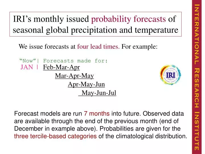
1. IRI’s monthly issued probability forecasts of seasonal global precipitation and temperature We issue forecasts at four lead times. For example: “Now”| Forecasts made for: JAN | Feb-Mar-Apr Mar-Apr-May Apr-May-Jun May-Jun-Jul Forecast models are run 7 months into future. Observed data are available through the end of the previous month (end of December in example above). Probabilities are given for the three tercile-based categories of the climatological distribution.

2. Forecasts of the climate The tercile category system: Below, near, and above normal Probability: 33% 33% 33% Below| Near | Below| Near | Above Below| Near | | || ||| ||||.| || | | || | | | . | | | | | | | | | | Data: 0 10 20 30 40 50 60 70 80 90 100 110 120 130 140 150 160 170 180 190 200 Rainfall Amount (mm) (30 years of historical data for a particular location & season)

3. Example of a typical climate forecast for a particular location & season Probability: 20% 35% 45% Below| Near | Below| Near | Above Below| Near | 0 10 20 30 40 50 60 70 80 90 100 110 120 130 140 150 160 170 180 190 200 Rainfall Amount (mm)

4. Example of a STRONGclimate forecast for a particular location & season Probability: 5% 25% 70% Below| Near | Below| Near | Above Below| Near | 0 10 20 30 40 50 60 70 80 90 100 110 120 130 140 150 160 170 180 190 200 Rainfall Amount (mm)

5. The probabilistic nature of climate forecasts Forecast distribution Historical distribution Above Below Historically, the probabilities of above and below are 0.33. Shifting the mean by half a standard-deviation and reducing the variance by 20% (red curve) changes the probability of below to 0.15 and of above to 0.53.

6. IRI DYNAMICAL CLIMATE FORECAST SYSTEM 2-tiered OCEAN ATMOSPHERE GLOBAL ATMOSPHERIC MODELS ECPC(Scripps) ECHAM4.5(MPI) CCM3.6(NCAR) NCEP(MRF9) NSIPP(NASA) COLA2 GFDL PERSISTED GLOBAL SST ANOMALY Persisted SST Ensembles 3 Mo. lead 10 POST PROCESSING MULTIMODEL ENSEMBLING 24 24 10 FORECAST SST TROP. PACIFIC: THREE (multi-models, dynamical and statistical) TROP. ATL, INDIAN (ONE statistical) EXTRATROPICAL (damped persistence) 12 Forecast SST Ensembles 3/6 Mo. lead 24 24 30 12 30 30 GFDL has 10 to PSST

7. IRI DYNAMICAL CLIMATE FORECAST SYSTEM 2-tiered OCEAN ATMOSPHERE MULTIPLE GLOBAL ATMOSPHERIC MODELS ECPC(Scripps) ECHAM4.5(MPI) CCM3.6(NCAR) NCEP(MRF9) NSIPP(NASA) COLA2 GFDL PERSISTED GLOBAL SST ANOMALY FORECAST SST TROP. PACIFIC:THREE scenarios: 1) CFS prediction 2) LDEO prediction 3) Constructed Analog prediction TROP. ATL, and INDIAN oceans CCA, or slowly damped persistence EXTRATROPICAL damped persistence

8. Collaboration on Input to Forecast Production Sources of the Global Sea Surface Temperature Forecasts Tropical Pacific Tropical Atlantic Indian Ocean Extratropical Oceans NCEP Coupled CPTEC Statistical IRI Statistical Damped PersistenceLDEO Coupled Constr Analogue Atmospheric General Circulation Models Used in the IRI's Seasonal Forecasts, for Superensembles Name Where Model Was Developed Where Model Is Run NCEP MRF-9 NCEP, Washington, DC QDNR, Queensland, AustraliaECHAM 4.5 MPI, Hamburg, Germany IRI, Palisades, New YorkNSIPP NASA/GSFC, Greenbelt, MD NASA/GSFC, Greenbelt, MDCOLA COLA, Calverton, MD COLA, Calverton, MD ECPC SIO, La Jolla, CA SIO, La Jolla, CA CCM3.6 NCAR, Boulder, CO IRI, Palisades, New York GFDL GFDL, Princeton, NJ GFDL, Princeton, NJ

9. Much of our predictability comes about due to ----- -----

11. Strong trade winds Westward currents, upwelling Cold east, warm west Convection, rising motion in west Weak trade winds Eastward currents, suppressed upwelling Warm west and east Enhanced convection, eastward displacement

12. NDJ Precipitation Probabilities associated with El Nino Empirical Approach (a good baseline by which to judge the more advanced methods “honest”) NDJ

13. Combining the Predictions of Seasonal Climate by Several Atmospheric General Circulation Models (AGCMs) into a Single Prediction.What is Done at IRI

14. Goals in Combining To combine the probability forecasts of several models, with relative weights based on the past performance of the individual models To assign appropriate forecast probability distribution: e.g. damp overconfident forecasts toward climatology

15. One Choice: Multiple Regression Multiple regression uses the predictions of 2 or more models, along with the corresponding observations, to derive a set of model weights that minimizes squared errors of the weighted predictions. Good feature: The actual skills of each model are taken into account, and also the overlap in sources of predictability. So, if two models have high skill in the same way or for the same reason, or if two good models are nearly identical, both of them do not get the same high weight. Bad features: (1) Random variations in the training sample are taken as seriously as the predictable part of the variability. This leads to overfitting, and poor results in real forecasts. The more predictors compared to the number of independent cases, the more severe this problem is. (2) Forecasts for conditions outside the range of the training sample may be dangerous. Note: A model’s weight does not necessarily describe its skill. In fact, negative weights can be seen for skillful models.

16. Another Choice: Simple Skill Weighting Here, the weights given to 2 or more models are determined by each model’s individual skill in forecasting observations. The skill may be a correlation or other measure. The weights are normalized so that their sum is 1. Good features: (1) The actual skills of each model are taken into account. (2) Overfitting is not as serious a problem here as it is in multiple regression. (3) Final forecast is always within the range of the individual forecasts. Bad feature: Duplication in the sources of skill is not checked. (Colinearity ignored.) So, if two good models are almost identical, both will be weighted strongly, even though the second one does not add much skill. A medium-skill model that has a unique source of skill will not influence the forecast enough. Note: A model’s weight is easily interpreted as being its skill.

17. Methods Used at IRI:(1) Bayesian Combination (2) Canonical Variate Combination Bayesian Combination Combine climatology forecast (“prior”) and an AGCM forecast, with its evidence of historical skill, to produce weighted (“posterior”) forecast probabilities, by maximizing the historical likelihood score.

18. Six GCM Precip. Forecasts, JAS 2000

19. RPSS Skill of Individual Models: JAS 1950-97

20. Probabilities and Uncertainty Climatological Probabilities GCM Probabilities k = tercile number t = forecast time m = no. ens members Above Normal 1/3 6/24 Tercile boundaries are identified for the models’ own climatology, by aggregating all years and ensemble members. This corrects overall bias. 1/3 Near-Normal 8/24 Below Normal 1/3 10/24

21. Bayesian Model Combination Combine climatology forecast (“prior”) and an AGCM forecast, with its evidence of historical skill, to produce weighted (“posterior”) forecast probabilities, by maximizing the historical likelihood score.

22. Aim to maximize the likelihood score k=tercile category t=year number The multi-year product of the probabilities that were hindcast for the category that was observed. (Could maximize other scores, such as RPSS) Prescribed, observed SST used to force AGCMs. Such simulations used in absence of ones using truly forecasted SST for at least half of AGCMs.

23. 1. Calibration of each model, individually, against climatology Optimize likelihood score k=tercile category (1,2, or 3) t=year number j=model number (1 to 7) w=weight for climo (c) or for model j PMMkt= weighted linear comb of Pjkt over all j, normalized by Σ(wj) 2. Calibration of the weighted model combination against climatol Optimize likelihood score where wMM uses wj proportional to results of the first step above

24. Algorithm used to maximize the designated score: Feasible Sequential Quadratic Programming (FSQP) “Nonmonotone line search for minimax problems” C M : TOTAL NUMBER OF CONSTRAINTS. C ME : NUMBER OF EQUALITY CONSTRAINTS. C MMAX : ROW DIMENSION OF A. MMAX MUST BE AT LEAST ONE AND GREATER C THAN M. C N : NUMBER OF VARIABLES. C NMAX : ROW DIMENSION OF C. NMAX MUST BE GREATER OR EQUAL TO N. C MNN : MUST BE EQUAL TO M + N + N. C C(NMAX,NMAX): OBJECTIVE FUNCTION MATRIX WHICH SHOULD BE SYMMETRIC AND C POSITIVE DEFINITE. IF IWAR(1) = 0, C IS SUPPOSED TO BE THE C CHOLESKEY-FACTOR OF ANOTHER MATRIX, I.E. C IS UPPER C TRIANGULAR. C D(NMAX) : CONTAINS THE CONSTANT VECTOR OF THE OBJECTIVE FUNCTION. C A(MMAX,NMAX): CONTAINS THE DATA MATRIX OF THE LINEAR CONSTRAINTS. C B(MMAX) : CONTAINS THE CONSTANT DATA OF THE LINEAR CONSTRAINTS. C XL(N),XU(N): CONTAIN THE LOWER AND UPPER BOUNDS FOR THE VARIABLES. C X(N) : ON RETURN, X CONTAINS THE OPTIMAL SOLUTION VECTOR. C U(MNN) : ON RETURN, U CONTAINS THE LAGRANGE MULTIPLIERS. THE FIRST C M POSITIONS ARE RESERVED FOR THE MULTIPLIERS OF THE M C LINEAR CONSTRAINTS AND THE SUBSEQUENT ONES FOR THE C MULTIPLIERS OF THE LOWER AND UPPER BOUNDS. ON SUCCESSFUL C TERMINATION, ALL VALUES OF U WITH RESPECT TO INEQUALITIES C AND BOUNDS SHOULD BE GREATER OR EQUAL TO ZERO.

25. Circumventing the effects of sampling variability • Sampling variability appears to be an issue: noisy weight distribution with large number of zero weights and some unity weights • Bootstrap the optimization, omitting contiguous 6-year blocks of the 48-yr time series • yields 43 samples of 42 years • shows the sampling variability of the likelihood over subsets of years • We average the weights across the samples

26. Example • Six GCMs’ Jul-Aug-Sep precipitation simulations • Training period: 1950–97 • Ensembles of between 9 and 24 members

27. Model Weights – initially, by individual model

28. Climatological Weights – Multi-model

29. Model Weights – after second (damping) step

30. Model Weights – step 2, and Averaged over Subsamples

31. For more spatially smooth results, the weighting of each grid point is averaged with that of its 8 neighbors, using binomial weighting. X X X X X X X X X

32. Climatological Weights

33. Combination Forecasts of July-Sept Precipitation After first stage only After second (damping) stage After sampling subperiods After spatial smoothing

34. ReliabilityJAS Precip., 30S-30N Above-Normal Below-Normal Bayesian Pooled Observed relative Freq. Observed relative Freq. Individual AGCM Forecast probability Forecast probability (3-model) from Goddard et al. 2003

35. RPSS Precip. from Roberson et al. (2004): Mon. Wea. Rev., 132, 2732-2744

36. RPSS 2-m Temp. from Roberson et al. (2004): Mon. Wea. Rev., 132, 2732-2744

37. Conclusions - Bayesian • The “climatological” (equal-odds) forecast provides a useful prior for combining multiple ensemble forecasts • Sampling problems become severe when attempting to combine many models from a short training period (“noisy weights”) • A two-stage process combines the models together according to a pre-assessment of each against climatology • Smoothing of the weights across data sub-samples and spatially appears beneficial

38. IRI’s forecasts use also a second consolidation scheme, whose result is averaged with the result of the Bayesian scheme. 1. Bayesian scheme 2. Canonical Variate scheme

39. Canonical Variate Analysis (CVA) • A number of statistical techniques involve calculating linear combinations (weighted sums) of variables. The weights are defined to achieve specific objectives: • PCA – weighted sums maximize variance • CCA – weighted sums maximize correlation • CVA – weighted sums maximize discrimination

40. Canonical Variate Analysis

41. Canonical Variate Analysis The canonical variates are defined to maximize the ratio of the between-category (separation between the crosses) to the within-category (separation of dots from like-colored crosses) variance.

42. Conclusion IRI is presently using a 2-tiered prediction system. It is interested in using fully coupled systems also, and is looking into incorporating those. Within its 2-tiered system it uses 4 SST prediction scenarios, and combines the predictions of 7 AGCMs. The merging of 7 predictions into a single one uses two multi-model ensemble systems: Bayesian and canonical variate. These give somewhat differing solutions, and are presently given equal weight.

43. Plan for Improvement of the Basic Forecast Product IRI plans to issue forecasts as probability density functions (pdfs) instead of just for the 3 tercile-based categories. From the pdfs, users can construct proba- bilities for any categories desired.

44. Skill results for IRI real-time climate forecasts from 1997-2001

45. Real-time Forecast Skill Goddard et al. 2003, Bull. Amer. Meteorol. Soc., 84, 1973-1796.

46. Real-time Forecast Skill Goddard et al. 2003, Bull. Amer. Meteorol. Soc., 84, 1973-1796.

47. Real-time Forecast Skill Goddard et al. 2003, Bull. Amer. Meteorol. Soc., 84, 1973-1796.

48. Real-time Forecast Skill Goddard et al. 2003, Bull. Amer. Meteorol. Soc., 84, 1973-1796.

50. RELIABILITY DIAGRAM Perfect reliability