Download
1 / 76
830 likes | 1.15k Views
Efficiency and Productivity. Ming-Miin YU OCT.6,2002. Outline. Introduction Economics Basic Concept Methodologies 1) Index Number 2) Least Square 3) DEA 4) SFA Conclusion. Introduction. What is Productivity? What is Efficiency? Productivity Technical Efficiency Production Frontier

E N D
Efficiency and Productivity Ming-Miin YU OCT.6,2002
Outline • Introduction • Economics • Basic Concept • Methodologies 1) Index Number2) Least Square3) DEA4) SFA • Conclusion
Introduction • What is Productivity? • What is Efficiency? • Productivity • Technical Efficiency • Production Frontier • Feasible Production Set • Scale Economies • Technical Change
Productivity Growth • Factors of Productivity Growth From One Year to Next Year • Efficiency Improvement • Technical Change • Scale Economies • Combination of Three Factors
Economics • Microeconomics Vs. Macroeconomics • Production Economics (PE) Vs. Consumption Economics(CE) • PE)Allocate resources such that Max. Profit or Min.costCE)Allocate income such that Max. utility or Min.expenditureHere we deal only with PE
Production Process Basic Concept • Production Technology gods input bads • Productivity = output / input
Feasible Production Set • represent a firm’s production technology by f(x). • All set on or below f(x) are feasible,while set above f(x) are infeasible inpresent technology. • f(x) is called production frontier.
Overall Efficiency • one output y was produced by a firm,which utilized two inputs,x1 and x2. • AA” is frontier,for firm D, technical efficiency=OC/OD • If prices of inputs are known,we candefine allocate efficiency by OB/OC(PP’ is isocost) • Overall eff.=TE*AE=(OC/OD)*(OB/OC)=OB/OD
Scale Effect • Distinction between techeff.&productivity • Both B and C areon frontier,henceboth are efficient. • But productivity ofC is greater than B (due to scale effect).
Methodologies • 1.Index number methods • 2.Least-square methods • 3.Data Envelopment Analysis (DEA) • 4.Stochastic Frontier Approach (SFP)
Frontier Non-Frontier Parametric Stochastic Frontier (SF) Econometric Methods (LS) Non-Parametric Data Envelopment Analysis (DEA) Index Numbers (TFP) Frontier and Non-FrontierParametric and Non-Parametric
Productivity Change • a ratio type Productivity Index P=[y]/[x] • Partial factor productivity vs.Total factor productivity P=[aggregrate Y]/[aggregrate X] P=[aggregrate Y]/[x1] • productivity change Pc=[Yt/Ys]/[Yt/Xs]
Decomposition of a Simple TFP Index • TFP Growth • Real Product in Period t • Homogeneous of degree
Decomposition of a Simple TFP Index • Change in Technical Efficiency • Technical Change • Effect of a Change in the Scale of Operations • Scale of Operations • Returns to Scale Parameter
Output and Input Quantity Index • utilizing only one input and produce one output? • multiple inputs and multiple outputs • Aggregrate Output :“output quantity index” • Aggregrate Input :“input quantity index”
Properties of Index Numbers • Test Approach1).Positivity.2).Continuity3).Proportionality4).Commensurability 5).Time-reversal test.6).Mean-value test7).Factor-reversal test.8).Circularity test(transitivity).
Tornqvist and CCD Index • Tornqvist index satisfies all properties list above except (7)&(8) • Index should satisfies transitivity, that is Ist=Isr *Irt(otherwise, can’t be compared • Caves,Christensen and Diewert(CCD,1982) convert Tornqvist indices into CCD indices as below,which satisfies transitivity:
Example: Tornqvist Index • Data for an artificial freight company • Input(quantity)year labor capital other1996 145 67 391997 166 75 391998 162 78 431999 178 89 422000 177 93 51
Input Price • Input(price)year labor capital other1996 39 100 1001997 41 110 971998 42 114 1031999 46 121 1192000 46 142 122
Output Quantity and Price • output(quantity) Price year O1 O2 O1 O2 1996 471 293 27 181997 472 290 28 17 1998 477 278 34 171999 533 277 32 202000 567 289 34 23
Tornqvist index number • Tornqvist index number:obsn output input TFP1 1.0000 1.0000 1.00002 0.9986 1.1007 0.90733 0.9960 1.1333 0.87884 1.0833 1.2340 0.87735 1.1468 1.3122 0.8740TFP down 13%
The Total Productivity of Canadian Railways • Tretheway,et.al (1997) “The Total Productivity of Canadian Railways” • The paper measured TFP of CanadianNational(CN)Railway & Canadian Pacific Rail(CP) by usingTornqvist TFP Index Number Method. • Input: labor,fuel&energy,way&structure, equipment,land,material&other. • Output:ton-km&pass-km.
The Result • The Result showed: • for CN,TFP growth rate (%) 1956-81 1981-91 11956-91 3.4 3.0 3.3 • for CP,TFP growth rate (%) 1956-81 1981-91 11956-91 3.4 2.7 3.2
2.Least-square methods • a firm’s production technology by y=f(x) • In practice, production function is never known. • One can estimate production functionby using Econometrics methods.
Specify a Functional Form • Before estimate,one should specify a functional form. • The most famous functional form probably is Cobb-Douglas Productionfunction. • The C-D function proposed in 1928 wasy=Ax1αx21-αx1:labor,x2:capital
Production Stages • Neoclassical Production Function: • 3 stagesstage 1:0~(MPP=APP)stage 2:(MPP=APP)~(MPP=0)stage 3:(MPP<0)
Restristions of CD Function • Because of its simplicity,C-D fn. has beenwidely used. • However,it can not represent 3-stage production function. • Besides,it imposed some assumption(such aselasticity of substitution=1) to function. • Many economists devoted to find a flexible functional form both from Primal and Dual.Note:flexible--no priori assumption.
Production and Cost Functions • Primal---estimate production fns.Dual----- estimate cost fns. • Specify function form (such as Translog, Quadratic,Leontif,etc.)and estimate it to get parameters. • For example,we specify Translog cost fn.as follows.
Translog Cost Function • lnC=α0+αLlnPL+αElnPE+αFlnPF+βYlnY+βQlnQ+γTT+δKlnK+(1/2)αLL(lnPL)2+αLElnPLlnPE+αLFlnPLlnPF+(1/2)αEE(lnPE)2+αEFlnPElnPF+(1/2)αFF(lnPF)2+θLYlnPLlnY+θEYlnPElnY+θFYlnPFlnY+λLQlnPLlnQ+λEQlnPElnQ+λFQlnPFlnQ+ρLTlnPLT+ρETlnPET+ρFTlnPFT+ηLKlnPLlnPk+ηEKlnPElnPk+ηFKlnPFlnPk +(1/2) βYY(lnY)2 +(1/2) βQQ(lnQ)2 +(1/2) γTT(T)2 +(1/2) δ KK(lnK)2 +τYTTlnY+μYKlnYlnK+ΨYQlnYlnQ+ωQTTlnQ+πQKlnQlnK+λTKTlnK
Properities • Where,C:cost; Y,Q:output;PL,PE,PF:input;T:time trend;K:fixed factor. • A well-behavior cost fn.satisfy someproperties,such as homogenous in degree 1,i.e. λC(y,p)=C(y, λp)therefore, one get:αL+αE+αF=1, αLL+αLE+αLF=0αEE+ αEL +αEF=0,αFF+αFL +αFE=0θLY+θEY+θFY=0, λLQ+λEQ+λFQ=0 ρLT+ρET+ρFT=0, ηLK+ηEK+ηFK=0
Shephard’s lemma • By using Shephard’s lemma,one getcost share eqs:
Parameter Estimation • Estimating the cost share eqs.and translog cost fn.silmutaneously,we getparameters.(using computer program) • Then,we can compute:1)Partial elasticities of substitution.2)Prices elasticities of factor demand.3)Economies of density.4)Productivity growth.
3.DEA • The two methods introduced above arenon-frontier. • Now,we turn the topic to Frontier. • The Frontier methods include:1)Data Envelopment Analysis(DEA)2)Stochastic Frontier Approach(SFA) • DEA involve mathematical programmingwhile SFA using econometric methods.
Distance Function • Farrell (1957)proposed:Economic eff.(EE)=Technical eff.(TE)*Allocative eff.(AE) • TE:given input,max.output,or given output,min.input. • AE:given input prices,optimal cost,or given output prices,optimal revenue.
Input Oriented DEA • Concept(input orientated) TEi=OQ/OP AEi=OR/OQ EEi=TEi*AEi =OR/OP
Output Orienrted DEA • Concept(output orientated) TEo=OA/OB AEo=OB/OC EEo=TEo*AEo =OA/OC
Constant Returns to Scale • For DMU Passume CRS,TEi=AB/APTEo=CP/CDTEi=TEo
Variable Returns to Scale • While in case of VRS,TEi is not equal toTEo • D • A B P • D
DEA Ratio Form • Primal Form for j = 1,2,…,n ur≧0 for r=1,2,…,s vi≧0 for i=1,2,…,m • Revised Form
Envelopment Form • Dual form and Technical Efficiency
Pure Technical Efficiency • SE = TE / PTE • OE = TE * AE = PTE * SE * AE…
Decomposition of Technical Efficiency 技術效率( )=MN/MA= 純粹技術效率( )=MB/MA= 規模效率( )=MN/MB=
Implement • Where thita is eff.score,Y,X are output and input of all DMU,yi,xi are output and input of i-th DMU,