Download
1 / 24
240 likes | 245 Views
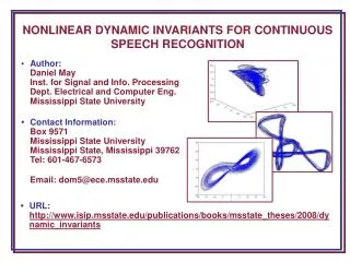
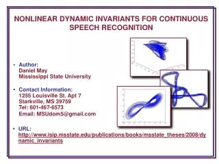
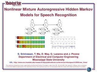
Nonlinear Dynamical Invariants for Speech Recognition. S. Prasad, S. Srinivasan , M. Pannuri, G. Lazarou and J. Picone Department of Electrical and Computer Engineering Mississippi State University

E N D
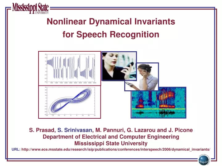
Nonlinear Dynamical Invariantsfor Speech Recognition S. Prasad, S. Srinivasan, M. Pannuri, G. Lazarou and J. Picone Department of Electrical and Computer Engineering Mississippi State University URL:http://www.ece.msstate.edu/research/isip/publications/conferences/interspeech/2006/dynamical_invariants/
Motivation • State-of-the-art speech recognition systems relying on linear acoustic models suffer from robustness problem. • Our goal: To study and use new features for speech recognition that do not rely on traditional measures of the first and second order moments of the signal. • Why nonlinear features? • Nonlinear dynamical invariants may be more robust (invariant) to noise. • Speech signals have both periodic-like and noise-like segments – similar to chaotic signals arising from nonlinear systems. • The motivation behind studying such invariants: to capture the relevant nonlinear dynamical information from the time series – something that is ignored in conventional spectral analysis.
Attractors for Dynamical Systems • System Attractor: Trajectories approach a limit with increasing time, irrespective of the initial conditions within a region • Basin of Attraction: Set of initial conditions converging to a particular attractor • Attractors: Non-chaotic (point, limit cycle or torus),or chaotic (strange attactors) • Example: point and limit cycle attractors of a logistic map (a discrete nonlinear chaotic map)
Strange Attractors • Strange Attractors: attractors whose shapes are neither points nor limit cycles. They typically have a fractal structure (i.e., they have dimensions that are not integers but fractional) • Example: a Lorentz system with parameters
Characterizing Chaos • Exploit geometrical (self-similar structure) aspects of an attractor or the temporal evolution for system characterization • Geometry of a Strange Attractor: • Most strange attractors show a similar structure at various scales, i.e., parts are similar to the whole. • Fractal dimensions can be used to quantify this self-similarity. • e.g., Hausdorff, correlation dimensions. • Temporal Aspect of Chaos: • Characteristic exponents or Lyapunov exponents (LE’s) - captures rate of divergence (or convergence) of nearby trajectories; • Also Correlation Entropy captures similar information. • Any characterization presupposes that phase-space is available. • What if only one scalar time series measurement of the system (and not its actual phase space) is available?
Reconstructed Phase Space (RPS): Embedding • Embedding: A mapping from a one-dimensional signal to an m-dimensional signal • Taken’s Theorem: • Can reconstruct a phase space “equivalent” to the original phase space by embedding with m ≥ 2d+1 (d is the system dimension) • Embedding Dimension: a theoretically sufficient bound; in practice, embedding with a smaller dimension is adequate. • Equivalence: • means the system invariants characterizing the attractor are the same • does not mean reconstructed phase space (RPS) is exactly the same as original phase space • RPS Construction: techniques include differential embedding, integral embedding, time delay embedding, and SVD embedding
Reconstructed Phase Space (RPS): Time Delay Embedding • Uses delayed copies of the original time series as components of RPS to form a matrix • m: embedding dimension, : delay parameter • Each row of the matrix is a point in the RPS
Reconstructed Phase Space (RPS) Time Delay Embedding of a Lorentz time series
Lyapunov Exponents • Quantifies separation in time between trajectories, assuming rate of growth (or decay) is exponential in time, as: • where J is the Jacobian matrix at point p. • Captures sensitivity to initial conditions. • Analyzes separation in time of two trajectories with close initial points • where is the system’s evolution function.
Correlation Integral • Measures the number of points within a neighborhood of radius, averaged over the entire attractor as: • where are points on the attractor (which has N such points). • Theiler’s correction: Used to prevent temporal correlations in the time series from producing an underestimated dimension. • Correlation integral is used in the computation of both correlation dimension and Kolmogorov entropy.
Fractal Dimension • Fractals: objects which are self-similar at various resolutions • Correlation dimension: a popular choice for numerically estimating the fractal dimension of the attractor. • Captures the power-law relation between the correlation integral of an attractor and the neighborhood radius of the analysis hyper-sphere as: • where is the correlation integral.
Kolmogorov-Sinai Entropy • Entropy: a well-known measure used to quantify the amount of disorder in a system. • Numerically, the Kolmogorov entropy can be estimated as the second order Renyi entropy ( ) and can be related to the correlation integral of the reconstructed attractor as: • where D is the fractal dimension of the system’s attractor, d is the embedding dimension and is the time-delay used for attractor reconstruction. • This leads to the relation: • In a practical situation, the values of and are restricted by the resolution of the attractor and the length of the time series.
Kullback-Leibler Divergence for Invariants • Measures discrimination information between two statistical models. • We measured invariants for each phoneme using a sliding window, and built an accumulated statistical model over each such utterance. • The discrimination information between a pair of models and is given by: • provides a symmetric divergence measure between two populations from an information-theoretic perspective. • We use as the metric for quantifying the amount of discrimination information across dynamical invariants extracted from different broad phonetic classes.
Experimental Setup • Collected artificially elongated pronunciations of several vowels and consonants from 4 male and 3 female speakers • Each speaker produced sustained sounds (4 seconds long) for three vowels (/aa/, /ae/, /eh/), two nasals (/m/, /n/) and three fricatives (/f/, /sh/, /z/). • The data was sampled at 22,050 Hz. • For this preliminary study, we wanted to avoid artifacts introduced by coarticulation. • Acoustic data to reconstructed phase space: using time delay embedding with a delay of 10 samples. (This delay was selected as the first local minimum of the auto-mutual information vs. delay curve averaged across all phones. • Window Size: 1500 samples.
Experimental Setup (Tuning Algorithmic Parameters) • Experiments performed to optimize parameters (by varying the parameters and choosing the value at which we obtain convergence) of estimation algorithm. • Embedding dimension for LE and correlation dimension: 5 • For Lyapunov exponent: • number of nearest neighbors: 30, • evolution step size: 5, • number of sub-groups of neighbors: 15. • For Kolmogorov entropy: • Embedding dimension of 15
Tuning Results: Lyapunov Exponents Lyapunov Exponents • For vowel: /ae/ For nasal: /m/ For fricative: /sh/ • In all three cases, the positive LE stabilizes at an embedding dimension of 5. • Positive LE much higher for fricative than nasals and vowels.
Tuning Results: Kolmogorov Entropy Kolmogorov Entropy • For vowel: /ae/ For nasal: /m/ For fricative: /sh/ • For vowels and nasals: Have stable behavior with embedding dimensions around 12-15. • For fricatives: Entropy estimate consistently increases with embedding dimension.
Tuning Results: Correlation Dimension Correlation Dimension • For vowel: /ae/ For nasal: /m/ For fricative: /sh/ • For vowels and nasals: Clear scaling region at epsilon = 0.75; Less sensitive to variations in embedding dimensions from 5-8. • For fricatives: No clear scaling region; more sensitive to variations in embedding dimension.
Experimental Results : KL Divergence - LE • Discrimination information for: • vowels-fricatives: higher • nasals-fricatives: higher • vowels-nasals: lower
Experimental Results : KL Divergence – Kolmogorov Entropy • Discrimination information for: • vowels-fricatives: higher • nasals-fricatives: higher • vowels-nasals: lower
Experimental Results : KL Divergence – Correlation Dimension • Discrimination information for: • vowels-fricatives: higher • nasals-fricatives: higher • vowels-nasals: lower
Summary and Future Work • Conclusions: • Reconstructed phase-space from speech data using Time Delay Embedding. • Extracted three nonlinear dynamical invariants (LE, Kolmogorov entropy, and Correlation Dimension) from embedded speech data. • Demonstrated the between-class separation of these invariants across8 phonetic sounds. • Encouraging results for speech recognition applications. • Future Work: • Study speaker variability with the hope that variations in the vocal tract response across speakers will result in different attractor structures. • Add these invariants as features for speech and speaker recognition.
Pattern Recognition Applet: compare popular linear and nonlinear algorithms on standard or custom data sets • Speech Recognition Toolkits: a state of the art ASR toolkit for testing the efficacy of these algorithms on recognition tasks • Foundation Classes: generic C++ implementations of many popular statistical modeling approaches • Resources
References • Kumar, A. and Mullick, S.K., “Nonlinear Dynamical Analysis of Speech,” Journal of the Acoustical Society of America, vol. 100, no. 1, pp. 615-629, July 1996. • Banbrook M., “Nonlinear analysis of speech from a synthesis perspective,” PhD Thesis, The University of Edinburgh, Edinburgh, UK, 1996. • Kokkinos, I. and Maragos, P., “Nonlinear Speech Analysis using Models for Chaotic Systems,” IEEE Transactions on Speech and Audio Processing, pp. 1098- 1109, Nov. 2005. • Eckmann, J.P. and Ruelle, D., “Ergodic Theory of Chaos and Strange Attractors,” Reviews of Modern Physics, vol. 57, pp. 617‑656, July 1985. • Kantz, H. and Schreiber T., Nonlinear Time Series Analysis, Cambridge University Press, UK, 2003. • Campbell, J. P., “Speaker Recognition: A Tutorial,” Proceedings of IEEE, vol. 85, no. 9, pp. 1437-1462, Sept. 1997.