Download
1 / 35
370 likes | 616 Views
Maximally Stable Extremal Regions and Extensions. Medical Image Processing Course. Loris Bazzani, PhD Student. Department of Computer Science, University of Verona, Italy, VIPS Lab. Supervisor: Prof. Vittorio Murino. Introduction. Maximally Stable Extremal Region

E N D
Maximally Stable Extremal Regions and Extensions Medical Image Processing Course Loris Bazzani, PhD Student Department of Computer Science, University of Verona, Italy, VIPS Lab. Supervisor: Prof. Vittorio Murino
Introduction • Maximally Stable Extremal Region • Maximally Stable Volume: 3D Extension • Segmentation of volumes • Maximally Stable Colour Region: RGB Extension • Objects of interest modeling • Conclusions
Outline • Maximally Stable Extremal Region • Maximally Stable Volume • Maximally Stable Colour Region • Conclusions
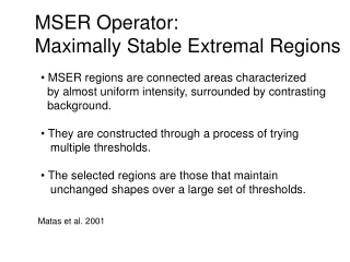
Maximally Stable Extremal Region(MSER) [Matas2002] • Set of all thresholdings of to a binary img: • MSER = connected region in with little size change across several thresholdings • Margin = the number of thresholds for which the region is stable
MSER (1) 3 1 4 2 5 [Images from Matas’ presentation]
Outline • Maximally Stable Extremal Region • Maximally Stable Volume • Maximally Stable Colour Region • Conclusions
Maximally Stable Volumes (MSV) [Donoser2006] New interpretation/formulation of MSER (2D): • Find the level sets of a connected, weighted graph • Node: pixel • Edge: connection relationship (e.g. 4-neghborhood) • Weight: pixel intensity • contains a set of nodes that have a weight above a given threshold • Build a component tree from a connected, weighted graph • Nodes: the connected components of • Edges: inclusion relationship between and
MSV (1) Extension to the third dimension: spatial or temporal • Find the level sets of a connected, weighted graph • Node: voxel • Edge: 3D connection relationship (e.g. 6-neghborhood) • Weight: voxel intensity • contains a set of nodes that have a weight above a given threshold • Build a component tree from a connected, weighted graph • Nodes: the connected volumes of • Edges: inclusion relationship between and
MSV (2) • A connected volume fulfills: • is the set of all boundary voxels of a volume • A connected volume is son of iff • i.e., an inclusion relationship between connected volumes
MSV (3) • MSVs are identified as the connected volumes with high stability: • Local minimum along the path to the root of the tree • Computation of the tree: • number of edges + nodes • inverse Ackermann function
3D segmentation (1) • Applied to simulated brain MR images • Size: , with different noise MSV detection result of brain segmentation. Images from [Donoser2006]
3D segmentation (2) 3D visualization of human brain, which was detected as a single MSV Images from [Donoser2006]
3D segmentation (3) • Applied to paper fiber network images • Sequences of cross-sectional images with max resolution of Images from [Donoser2006]
3D segmentation (4) Segmented fiber detected as MSV Images from [Donoser2006]
Outline • Maximally Stable Extremal Region • Maximally Stable Volume • Maximally Stable Colour Region • Conclusions
Maximally Stable Colour Region (MSCR) [Forssen2007] • Novel colour-based affine covariant region detector • Extension of the MSER to colour • Look at successive time-steps of an aggloramerative clustering of image pixel, based on proximity and similarity on colour • Modelling of the distribution of edge magnitudes • Novel edge significance measure based on a Poisson image noise model • Perform better than MSER and other state-of-the-art blob detectors • Applications: 3D object recognition and view matching Original set of images MSCR representation
MSCR (1) • Evolution process over the image that successively clusters neighbouring pixels with similar colours • For each time step , the evolution is a map of labels • Any two positions are connected by a path of distances which are smaller than
MSCR (2) Evolution Process with agglomerative clustering • is all zeroes • is constructed from by assigning new regions to all pair of pixel with • If one pixel of the pair already belongs to a region, the non-assigned pixel is appended to the region • If both pixels belong to regions the corresponding regions are merged
MSCR (3) • How the distance is defined: • Sensors count the number of photons • Noise follows the discrete Poisson distribution • For high , good approximation is a Gaussian: • Measure of edge significance: probability that a pixel has a larger mean than its neighbour: Chi-squared distance
MSCR (4) • Dynamically adapt the threshold : • Linearly increasing: very fast image evolution in the beginning and very slow at the end of the evolution • Change according to the inverse Cumulative Distribution Function (CDF) • Observation: edge significance measure follows a Chi-squared distribution: • Evolution thresholds:
MSCR (5) • Detecting stable regions: • For each region in the label image, we store the area and the distance threshold • When the area increases more than a threshold , and are re-initialized • The slope of the area and distance function is used for the detection if is the best (smallest), the region is stored
MSCR (6) • Descriptor for the MSCRs: • Region area • Centroid • Inertia Matrix • Average colour • These measures define an approximating ellipse for the detected region as:
Tracking-by-detection (1) • Tracking: spatial and temporal localization of a mobile object in an environment monitored by sensor(s) • Multi-target (MTT): keeping the identity of different targets • Reliable: insensible to noise and occlusions • Detection: identify all the objects of interest into the image • Tracking-by-detection: • targets are detected for every frame • IDs are associated from frame (t-1) to frame (t), with a data association process
Tracking-by-detection (2) • Tracking-by-detection using the MSCR descriptor • Our method extracts the MSCR from the foreground of the detected objects • We define a distance measurement in order to compare the objects at time (t-1) with the objects at time (t) • For each pair of blobs, we have: • Color distance: • y distance: • Distance between the objects : Euclidean distance
Qualitative Results (1) Image in the database Probe Image MSCR MSCR
Quantitative Results Tagging error Rate for each t Tagging error Rate for each N of ped Total Tagging Success Rate
Person Re-identification (1) • Multi-camera scenario with (non-)overlapping fields of View (FoV) • Objective: recognize an object, when it is being seen in different FoV • Challenging problem with non-overlapping FoV • Idea: • Keep a database of all the history of the seen objects • Once a new object enters in the scene, the method retrieves the IDs of the object from the database (if it is being seen before) • If the object is not in the database, a new ID is given to it and it is added to the database
Person Re-identification (2) • The method is the same used for tracking-by-detection problem • Compute the distance • Extraction of part-based HSV histogram • Divide the image in three parts: legs, torso, head • Compare the hist. of each part using the Bhattacharyya distance • MSCR and HSV hist. distance are combined:
Quantitative Results (1) • Evaluation in term of: • Cumulative Matching Characteristic (CMC): represents the expectation of finding the correct match in the top n matches • Synthetic Recognition Rate (SRR): represents the probability that any of the m best matches is correct • Using challenging publicly available datasets: VIPeR and iLIDS Dataset • pose variation and shape deformation • illumination changes, camera movement, and occlusions • noise and blurring
Quantitative Results (2) VIPeR dataset CMC SRR Thank to M. Farenzena and C. Cristani
Quantitative Results (2) iLIDS dataset Matching CMC Thank to M. Farenzena and C. Cristani
Conclusions • Two extensions of the MSER feature had been discussed • MSV that deals with 3D segmentation and modeling of medical images • MSCR that deals with hard problems in very different applications: tracking-by-detection, and person re-identification • MSER and extensions seem to be good features for representing and segmenting of object of interest in different kind of application
Thanks!Questions? References [Matas2002] J. Matas, O. Chum, M. Urban and T. Pajdla, Robust Wide Baseline Stereo from Maximally Stable Extremal Regions, In BMVC, 2002. [Donoser2006] M. Donoser and H. Bischrof, 3D Segmentation by Maximally Stable Volumes (MSVs), In ICPR, 2006. [Forssen2007] P. Forssen, Maximally Stable Colour Regions for Recognition and Matching, In CVPR, 2007.