Download
1 / 293

E N D
INTRODUCTION • Amplitude modulation (AM) radio is a commonplace technology today, and is standard in any type of commercial stereo device. Because of the low cost of the parts necessary to implement AM transmission and the simplicity of the underlying technology, using amplitude modulations is a cheap and effective way to perform many tasks that require wireless communication. • The most well-known application of an AM transmitter is in radio. Am radio receivers are available in numerous devices, from automobile stereos to clock radios. However, the usage of AM transmitters is not restricted to professional radio stations
Transmit information bearing (message) or baseband signal (voice music) through a communication channel • Baseband = is a range of frequency signal to be transmitted. eg: Audio (0 - 4 kHz), Video (0 - 6 MHz). • Communication channel: • Transmission without frequency shifting. • Transmission through twisted pair cable, coaxial cable and fiber optic cable. • Significant power for whole range of frequencies. • Not suitable for radio/microwave and satellite communication. • Carrier communication • Use technique of modulation to shift the frequency. • Change the carrier signal characteristics (amplitude, frequency and phase) following the modulating signal amplitude. • Suitable for radio/microwave and satellite communication.
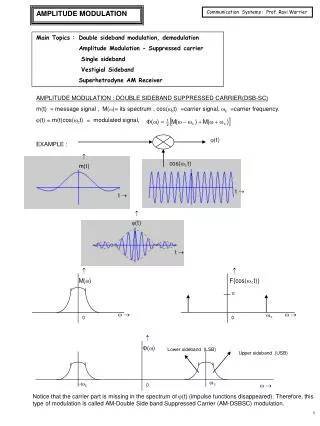
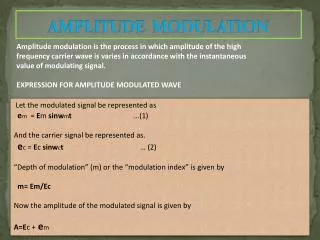
the instantaneous amplitude of a carrier wave is varied in accordance with the instantaneous amplitude of the modulating signal. Main advantages of AM are small bandwidth and simple transmitter and receiver designs. Amplitude modulation is implemented by mixing the carrier wave in a nonlinear device with the modulating signal. This produces upper and lower sidebands, which are the sum and difference frequencies of the carrier wave and modulating signal. • The carrier signal is represented by • c(t) = A cos(wct) • The modulating signal is represented by • m(t) = B sin(wmt) • Then the final modulated signal is • [1 + m(t)] c(t) • = A [1 + m(t)] cos(wct) • = A [1 + B sin(wmt)] cos(wct) • = A cos(wct) + A m/2 (cos((wc+wm)t)) + A m/2 (cos((wc-wm)t))
Single sideband suppressed carrier (ssbsc) • Form of amplitude modulation(AM); carrier is suppressed (typically 40 – 60dB below carrier) • For short we call it SSB since the carrier is usually not transmitted • Advantages • Conservation of spectrum space (SSB signal occupies only half the band of DSB signal) • The useful power output of the transmitter is greater since the carrier is not amplified • SSB receiver is quieter due to the narrower bandwidth (receiver noise is a function of bandwidth) • Disadvantages • The carrier must be reinserted the receiver, to down convert the sideband back to the original modulating audio • Carrier must be reinserted with the same frequency and phase it would have if it were still present • This is why clarity control on a CB radio is so fiddly, if carrier not inserted correctly the received output will be like donald duck voice.
SSB-LSB SIGNAL SSB-USB SIGNAL
SSB-LSB signal SSB-USB signal • SSB signal frequency spectrum
Hartley modulator • A direct approach for creating a single sideband AM signal (SSB-AM) is to remove either the upper or lower SB by filtering the DSBSC-AM signal (frequency discriminator method) SSB modulator using the frequency discrimination approach Magnitude spectra : (a) baseband ; (b) DSBSC-AM; (c) upper SSB; (d) lower SSB
Quadrature modulator can be used to create a SSB-AM signal by selecting the quadrature signal to coherently cancel either the upper /lower SB from the inphase channel • SSB-AM signal given: • Using the minus sign in equation (1) results in upper SSB,whereas selection of the plus sign yields lower SSB • The hilbert transform is a wideband -90° phase shifter (1) (2)
Hartley modulator for SSB; -sign gives upper SSB, +sign gives lower SSB
Angle Modulation – Frequency Modulation Consider again the general carrier represents the angle of the carrier. There are two ways of varying the angle of the carrier. • By varying the frequency, c – Frequency Modulation. • By varying the phase, c – Phase Modulation 1
Frequency Modulation In FM, the message signal m(t) controls the frequency fcof the carrier. Consider the carrier then for FM we may write: FM signal ,where the frequency deviation will depend on m(t). Given that the carrier frequency will change we may write for an instantaneous carrier signal and fi is the instantaneous where iis the instantaneous angle = frequency. 2
Frequency Modulation then Since i.e. frequency is proportional to the rate of change of angle. If fcis the unmodulated carrier and fm is the modulating frequency, then we may deduce that fcis the peak deviation of the carrier. Hence, we have ,i.e. 3
Frequency Modulation After integration i.e. Hence for the FM signal, 4
Frequency Modulation The ratio is called the Modulation Index denoted by i.e. Note – FM, as implicit in the above equation for vs(t), is a non-linear process – i.e. the principle of superposition does not apply. The FM signal for a message m(t) as a band of signals is very complex. Hence, m(t) is usually considered as a 'single tone modulating signal' of the form 5
Frequency Modulation The equation may be expressed as Bessel series (Bessel functions) where Jn() are Bessel functions of the first kind. Expanding the equation for a few terms we have: 6
FM Signal Spectrum. The amplitudes drawn are completely arbitrary, since we have not found any value for Jn() – this sketch is only to illustrate the spectrum. 7
Generation of FM signals – Frequency Modulation. • An FM demodulator is: • a voltage-to-frequency converter V/F • a voltage controlled oscillator VCO In these devices (V/F or VCO), the output frequency is dependent on the input voltage amplitude. 8
V/F Characteristics. Apply VIN , e.g. 0 Volts, +1 Volts, +2 Volts, -1 Volts, -2 Volts, ... and measure the frequency output for each VIN . The ideal V/F characteristic is a straight line as shown below. fc, the frequency output when the input is zero is called the undeviated or nominal carrier frequency. is called the Frequency Conversion Factor, The gradient of the characteristic denoted by per Volt. 9
V/F Characteristics. Consider now, an analogue message input, As the input m(t) varies from the output frequency will vary from a maximum, through fc, to a minimum frequency. 10
V/F Characteristics. For a straight line, y = c + mx, where c = value of y when x = 0, m = gradient, hence we may say and when VIN = m(t) ,i.e. the deviation depends on m(t). Considering that maximum and minimum input amplitudes are +Vm and -Vm respectively, then on the diagram on the previous slide. The peak-to-peak deviation is fmax – fmin, but more importantly for FM the peak deviation fc is Peak Deviation, Hence, Modulation Index, 11
Summary of the important points of FM • In FM, the message signal m(t) is assumed to be a single tone frequency, • The FM signal vs(t) from which the spectrum may be obtained as where Jn() are Bessel coefficients and Modulation Index, • Hz per Volt is the V/F modulator, gradient or Frequency Conversion Factor, per Volt • is a measure of the change in output frequency for a change in input amplitude. • Peak Deviation (of the carrier frequency from fc) 12
FM Signal Waveforms. The diagrams below illustrate FM signal waveforms for various inputs At this stage, an input digital data sequence, d(t), is introduced – the output in this case will be FSK, (Frequency Shift Keying). 13
FM Signal Waveforms. the output ‘switches’ between f1 and f0. Assuming 14
FM Signal Waveforms. The output frequency varies ‘gradually’ from fc to (fc + Vm), through fc to (fc - Vm) etc. 15
FM Signal Waveforms. If we plot fOUT as a function of VIN: In general, m(t) will be a ‘band of signals’, i.e. it will contain amplitude and frequency variations. Both amplitude and frequency change in m(t) at the input are translated to (just) frequency changes in the FM output signal, i.e. the amplitude of the output FM signal is constant. Amplitude changes at the input are translated to deviation from the carrier at the output. The larger the amplitude, the greater the deviation. 16
FM Signal Waveforms. Frequency changes at the input are translated to rate of change of frequency at the output. An attempt to illustrate this is shown below: 17
FM Spectrum – Bessel Coefficients. The FM signal spectrum may be determined from The values for the Bessel coefficients, Jn() may be found from graphs or, preferably, tables of ‘Bessel functions of the first kind’. 18
FM Spectrum – Bessel Coefficients. Jn() = 2.4 = 5 , hence the In the series for vs(t), n = 0 is the carrier component, i.e. n = 0 curve shows how the component at the carrier frequency, fc, varies in amplitude, with modulation index . 19
FM Spectrum – Bessel Coefficients. Hence for a given value of modulation index , the values of Jn() may be read off the graph and hence the component amplitudes (VcJn()) may be determined. A further way to interpret these curves is to imagine them in 3 dimensions 20
Examples from the graph = 0: When = 0 the carrier is unmodulated and J0(0) = 1, all other Jn(0) = 0, i.e. = 2.4: From the graph (approximately) J0(2.4) = 0, J1(2.4) = 0.5, J2(2.4) = 0.45 and J3(2.4) = 0.2 21
Significant Sidebands – Spectrum. As may be seen from the table of Bessel functions, for values of n above a certain value, the values of Jn() become progressively smaller. In FM the sidebands are considered to be significant if Jn() 0.01 (1%). Although the bandwidth of an FM signal is infinite, components with amplitudes VcJn(), for which Jn() < 0.01 are deemed to be insignificant and may be ignored. Example: A message signal with a frequency fm Hz modulates a carrier fc to produce FM with a modulation index = 1. Sketch the spectrum. 22
Significant Sidebands – Spectrum. As shown, the bandwidth of the spectrum containing significant components is 6fm, for = 1. 23
Significant Sidebands – Spectrum. The table below shows the number of significant sidebands for various modulation indices () and the associated spectral bandwidth. e.g. for = 5, 16 sidebands (8 pairs). 24
Carson’s Rule for FM Bandwidth. An approximation for the bandwidth of an FM signal is given by BW = 2(Maximum frequency deviation + highest modulated frequency) Carson’s Rule 25
Narrowband and Wideband FM Narrowband FM NBFM From the graph/table of Bessel functions it may be seen that for small , ( 0.3) there is only the carrier and 2 significant sidebands, i.e. BW = 2fm. FM with 0.3 is referred to as narrowband FM (NBFM) (Note, the bandwidth is the same as DSBAM). Wideband FM WBFM For > 0.3 there are more than 2 significant sidebands. As increases the number of sidebands increases. This is referred to as wideband FM (WBFM). 26
VHF/FM VHF/FM (Very High Frequency band = 30MHz – 300MHz) radio transmissions, in the band 88MHz to 108MHz have the following parameters: fm Max frequency input (e.g. music) 15kHz Deviation 75kHz Modulation Index 5 For = 5 there are 16 sidebands and the FM signal bandwidth is 16fm = 16 x 15kHz = 240kHz. Applying Carson’s Rule BW = 2(75+15) = 180kHz. 27
Comments FM • The FM spectrum contains a carrier component and an infinite number of sidebands • at frequencies fcnfm (n = 0, 1, 2, …) FM signal, • In FM we refer to sideband pairs not upper and lower sidebands. Carrier or other • components may not be suppressed in FM. • The relative amplitudes of components in FM depend on the values Jn(), where thus the component at the carrier frequency depends on m(t), as do all the other components and none may be suppressed. 28
Comments FM • Components are significant if Jn() 0.01. For <<1 ( 0.3 or less) only J0() and • J1() are significant, i.e. only a carrier and 2 sidebands. Bandwidth is 2fm, similar to • DSBAM in terms of bandwidth - called NBFM. means that a large bandwidth is required – called • Large modulation index WBFM. • The FM process is non-linear. The principle of superposition does not apply. When • m(t) is a band of signals, e.g. speech or music the analysis is very difficult • (impossible?). Calculations usually assume a single tone frequency equal to the • maximum input frequency. E.g.m(t) band 20Hz 15kHz, fm = 15kHz is used. 29
Power in FM Signals. From the equation for FM we see that the peak value of the components is VcJn() for the nth component. Single normalised average power = then the nth component is Hence, the total power in the infinite spectrum is Total power 30
Power in FM Signals. By this method we would need to carry out an infinite number of calculations to find PT. But, considering the waveform, the peak value is Vc, which is constant. Since we know that the RMS value of a sine wave is and power = (VRMS)2 then we may deduce that Hence, if we know Vc for the FM signal, we can find the total power PT for the infinite spectrum with a simple calculation. 31
Power in FM Signals. Now consider – if we generate an FM signal, it will contain an infinite number of sidebands. However, if we wish to transfer this signal, e.g. over a radio or cable, this implies that we require an infinite bandwidth channel. Even if there was an infinite channel bandwidth it would not all be allocated to one user. Only a limited bandwidth is available for any particular signal. Thus we have to make the signal spectrum fit into the available channel bandwidth. We can think of the signal spectrum as a ‘train’ and the channel bandwidth as a tunnel – obviously we make the train slightly less wider than the tunnel if we can. 32
Power in FM Signals. However, many signals (e.g. FM, square waves, digital signals) contain an infinite number of components. If we transfer such a signal via a limited channel bandwidth, we will lose some of the components and the output signal will be distorted. If we put an infinitely wide train through a tunnel, the train would come out distorted, the question is how much distortion can be tolerated? Generally speaking, spectral components decrease in amplitude as we move away from the spectrum ‘centre’. 33
Power in FM Signals. In general distortion may be defined as With reference to FM the minimum channel bandwidth required would be just wide enough to pass the spectrum of significant components. For a bandlimited FM spectrum, let a = the number of sideband pairs, e.g. for = 5, a = 8 pairs (16 components). Hence, power in the bandlimited spectrum PBL is = carrier power + sideband powers. 34
Power in FM Signals. Since Distortion Also, it is easily seen that the ratio = 1 – Distortion i.e. proportion pf power in bandlimited spectrum to total power = 35
Example Consider NBFM, with = 0.2. Let Vc = 10 volts. The total power in the infinite spectrum = 50 Watts, i.e. = 50 Watts. From the table – the significant components are or 99% of the total power i.e. the carrier + 2 sidebands contain 36
Example or 1%. Distortion = Actually, we don’t need to know Vc, i.e. alternatively Distortion = (a = 1) D = Ratio 37
FM Demodulation –General Principles. • An FM demodulator or frequency discriminator is essentially a frequency-to-voltage • converter (F/V). An F/V converter may be realised in several ways, including for • example, tuned circuits and envelope detectors, phase locked loops etc. • Demodulators are also called FM discriminators. • Before considering some specific types, the general concepts for FM demodulation • will be presented. An F/V converter produces an output voltage, VOUT which is • proportional to the frequency input, fIN. 38