Download
1 / 25
250 likes | 356 Views
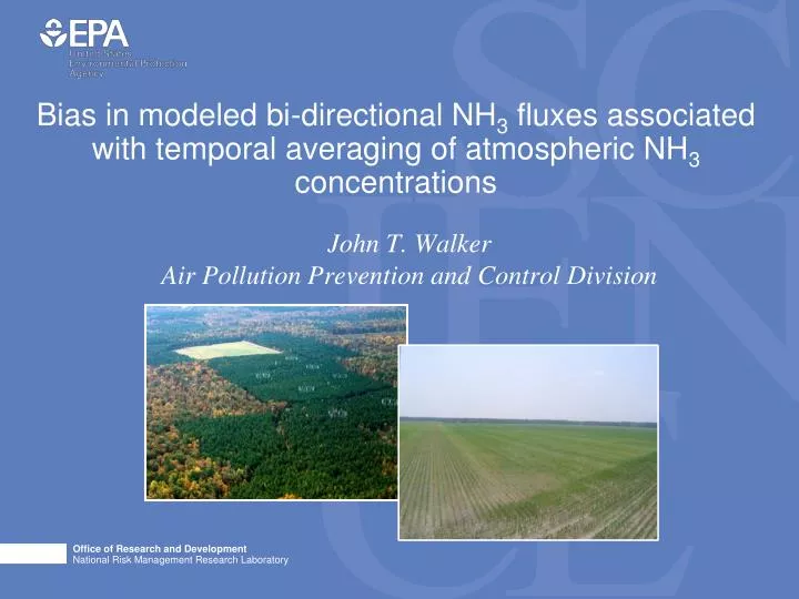
Bias in modeled bi-directional NH 3 fluxes associated with temporal averaging of atmospheric NH 3 concentrations . John T. Walker Air Pollution Prevention and Control Division. Introduction.

E N D
Bias in modeled bi-directional NH3 fluxes associated with temporal averaging of atmospheric NH3 concentrations John T. Walker Air Pollution Prevention and Control Division
Introduction • Direct flux measurements of NH3 are expensive, labor intensive, and require detailed supporting measurements of soil, vegetation, and atmospheric chemistry for interpretation and model parameterization. • It is therefore often necessary to infer fluxes by combining measurements of atmospheric concentrations, meteorology, and surface chemistry within a suitable air-surface exchange model. • Two-week integrated NH3 air concentrations are currently measured using passive diffusion samplers at ≈ 65 sites within the U.S. as part of the NADP Ammonia Monitoring Network (AMON). • Ideally, these measurements could be used to estimate NH3 fluxes in a manner similar to CASTNet, in which deposition is estimated by combining hourly meteorological measurements with weekly integrated air concentrations.
Introduction • Estimation of site specific NH3 fluxes from AMON data and other time-integrated monitoring data will require: • Identification of a suitable air-surface exchange model • Collection of necessary supporting data to parameterize the model • Measurements of soil and vegetation NH4+ and H+ concentrations are required to predictsurface compensation points • Evaluation of model performance • The accuracy of the modeled flux will comprise errors resulting from: • the inability of the model to accurately simulate the flux • the use of time-integrated data, rather than hourly data, to drive the model
Introduction • The use of time-integrated (temporally averaged) air concentrations may produce error in the modeled NH3 flux due to: • bias in the air concentration at the hourly time scale, which directly biases the flux • covariance between the atmospheric concentration and other variables that drive the flux • This study investigates temporal averaging of the NH3 air concentration as a source of error in modeled fluxes using a series of simulations in which temporally aggregated fluxes (seasonal and annual) derived from hourly versus time-integrated air concentrations are compared for a range of atmospheric and surface conditions. • Analysis of the ability of the air-surface model to accurately reproduce hourly fluxes by comparison to field data is forthcoming.
Background – NH3 Compensation Point Ammonia may be emitted from or deposited to vegetation, soil, and water, depending on the ratio of the atmospheric NH3 concentration to the compensation point of the underlying surface. Ammonia air-surface exchange processes are “bi-directional”. The compensation point (c) is, in general, governed by the nitrogen status and acidity of the exchange surface. cair = 1.5 mg NH3 m-3 NH3 emission cground>cair High NH4+, pH cground = 10 mg NH3 m-3 Fertilized Soil The NH3 emission potential of fertilized soil is a function of soil NH4+ and H+ concentrations, water content, and temperature. Compensation point Emission potential ()
Methods – Air/Surface Exchange Model Two-layer bi-directional resistance model of NH3 air-surface exchange parameterized according to Massad et al., 2010 Atmosphere Resistances Aerodynamic (Ra) Boundary layer (Rb) In-canopy (Rac, Rbg) Stomatal (Rs) Cuticular (Rw) Compensation points Canopy (zo) Stomatal(s) Ground (g) Fluxes Net canopy-scale (Ft) Stomatal (Fs) Cuticular (Fw) Foliage (Ff) Ground (Fg) Foliage (cuticle and stomata) Ground (soil and litter)
The goal of this modeling exercise is to illustrate the characteristics of bias between hourly and temporally averaged NH3 fluxes and to assess the potential magnitude of this bias in seasonal and annual aggregate fluxes. • To establish a range of flux conditions, the following scenarios for natural ecosystems were investigated: • Low soil/vegetation emission potential (= 25) • Net deposition to the ecosystem during all seasons • Intermediate soil/vegetation emission potential ( = 300) • Net emission only during summer • High soil/vegetation emission potential ( = 700) • Net deposition only during winter Methods – Model Scenarios
For each scenario, fluxes are calculated for each successive two week period over a full year by applying: a) hourly concentrations and hourly meteorology and b) the corresponding two-week average concentration and hourly meteorology. • A temporal averaging period of two weeks was chosen for consistency with the AMON sampling protocol, in which two week integrated air concentrations are measured by passive diffusion sampler. • Fluxes derived from hourly concentrations are compared to fluxes derived from two-week average concentrations at seasonal and annual scales. • Seasonal and annual total fluxes are calculated by summing hourly values. • The primary metric of comparison is % bias relative to the flux derived from hourly air concentrations. • Example: An annual flux of -2.0 kg ha-1 yr-1 (deposition) derived from two-week average concentrations has: • +100% bias relative to a flux of -1.0 kg ha-1 yr-1 derived from hourly concentrations (i.e., higher deposition) • - 50% bias relative to a flux of -4.0 kg ha-1 yr-1 derived from hourly concentrations (i.e., lower deposition) Methods – Model Scenarios and Comparison of Fluxes
Hourly meteorological data from the Bondville, IL AMON site were used for all simulations. Date include air temperature, wind speed, standard deviation of the wind direction, relative humidity, and global solar radiation. Parameterization of atmospheric resistances for the flux model follows Massad et al. (2010) and Walker et al. (2008; 2013). • With respect to atmospheric NH3, fluxes will be regulated by both the magnitude and temporal variability of the air concentration. • Air concentration magnitude and seasonal variability are based on AMON observations from sites (N = 54) that have a record of at least one full year. • Diurnal variability is simulated based on hourly datasets collected in agricultural and non-agricultural rural locations (Walker et al., 2006; 2012; 2013). Methods – Meteorology and NH3 Air Concentrations
AMON statistics • 54 sites with at least one year of • observations • Statistics derived from distribution • of site-wise means • Seasonal Variability • Ratios of individual observations • to the corresponding site mean • were averaged by month • across all sites to establish the • general seasonal pattern. • The ambient NH3 concentration • (a) with a seasonal cycle was • modeled as: Results – Air Concentrations
Diurnal Variability • Simulations of the diurnal variability of NH3 air concentrations are based on patterns observed at agricultural (Lillington, NC and Warsaw, NC) and non-agricultural rural sites. • At Duke Forest, hereafter referred to as Profile A, concentrations peak near mid-day, most likely reflecting the temperature dependence of the surface compensation point. • In agricultural regions, hereafter referred to as Profile B, boundary layer dynamics and surface NH3 emissions produces a bimodal profile with a pronounced morning peak and afternoon minimum. • Similar to seasonal variability, diurnal variability is also simulated using a wave function. Results – Air Concentrations
Low Diurnal profile A Cumulative annual flux Flux is negative (i.e., deposition) during all periods under this scenario. Over the course of a year, the cumulative flux derived from 2-week integrated air concentrations is ≈ 4% lower than the flux derived from hourly concentrations. Results – Flux Comparison Flux seasonality is driven by seasonality in the air concentration Bias generally low but varies seasonally
Low Diurnal profile A Relative to the hourly air concentration, the 2-week average concentration overestimates at night and underestimates during the day. Results – Processes that influence bias During winter, the overestimated concentration at night produces an overestimation of cuticular deposition, which dominates the flux budget. This drives the overall winter bias between total fluxes. During summer, the underestimated concentration during the day produces an underestimation of stomatal deposition, which dominates the flux budget. This drives the overall summer bias between total fluxes.
Intermediate Diurnal profile A Cumulative annual flux The net deposition flux is generally lower in this scenario because the air concentration is closer to the compensation point. The cumulative flux derived from 2-week average air concentrations is ≈ 11% lower than the flux derived from hourly concentrations. Results – Flux Comparison Temperature dependence of the compensation point produces net emission during summer. Bias displays large variability over the course of a year.
Intermediate Diurnal profile A Relative to the hourly air concentration, the 2-week average underestimates during the day. Results – Processes that influence bias During spring, the underestimated concentration during the day produces stomatal and ground emission fluxes, which dominate the flux budget. This drives the overall spring bias between total fluxes. During summer, the underestimated concentration during the day produces an overestimation of stomatal and ground emission, which dominates the flux budget. This drives the overall summer bias between total fluxes.
High Diurnal profile A Cumulative annual flux Flux is positive (i.e., emission) with the exception of winter. Over the course of a year, the cumulative flux derived from two-week integrated air concentrations is ≈ 5% higher than the flux derived from hourly concentrations. Results – Flux Comparison Fluxes derived from 2-week average concentrations are larger than those derived from hourly concentrations during all seasons.
High emission potential Profile A Relative to the hourly air concentration, the 2-week average underestimates during the day. Results – Sources of flux bias The underestimated concentration during the day produces an overestimation of stomatal and ground emission fluxes, which dominate the flux budget. This drives the overall spring and summer bias between total fluxes.
How much of the bias between fluxes is due to correlation between the hourly air concentration and variables that drive the vertical exchange rate? Results – Sources of Flux Bias • For species that are exchanged with the surface unidirectionally, such as SO2 and HNO3, the hourly flux is equal to the product of air concentration (a) and deposition velocity (Vd): • F = a Vd • which averaged over time (two weeks, for example) becomes: • where the overbar denotes averaging of the hourly values. The average flux may also be expressed as • where the first term on the right represents the product of the mean concentration and deposition velocity and the second term represents the average product of the hourly deviations from the mean. • If concentration and deposition velocity are uncorrelated, then the 2-week integrated flux may be calculated from 2-week average concentration and deposition velocity. • If the two are correlated, the 2-week average flux will be underestimated.
Unfortunately this approach does not work for NH3, which is exchanged bi-directionally as a function of a non-zero surface concentration (compensation point). Results – Sources of Flux Bias In the previous example, Vd is not a function of a. The air concentration is physically independent of the exchange velocity. For NH3, where o, the surface compensation point,is a function of both the air concentration (a) and the aerodynamic resistance (Ra). In this case, the air concentration and exchange velocity are not independent. As a first approximation, however, we can examine the correlation between the air concentration and the maximum possible exchange velocity (Vemax) established by the aerodynamic resistance: Correlation between hourlya and Vemax represents covariance between the air concentration and degree of turbulent mixing, a primary driver of the flux. This allows us to examine the potential contribution of covariance to the total bias between fluxes derived from hourly versus 2-week average concentrations described above.
Results – Sources of Flux Bias Values represent medians of bins containing 100 observations. The air concentration and maximum exchange velocity are not correlated at night but display relatively strong correlation during the day.
Results – Bias versus flux magnitude For net deposition, the flux estimated from 2-week average concentrations underestimates relative the flux derived from hourly concentrations. Net Emission For net emission, the flux estimated from 2-week average concentrations overestimates relative the flux derived from hourly concentrations. Net Deposition Bias increases non-linearly as the net flux changes from emission to deposition. Bias exceeds 20% for fluxes < 0.2 kg NH3 ha-1 yr-1.
At sites where the diurnal NH3 concentration peaks near mid-day, the 2-week integrated air concentration will be biased high at night and low during the day. • This bias in concentration produces an overestimate of cuticular deposition at night and an underestimate of stomatal and ground deposition during the day at sites with low surface emission potential. • At sites with higher surface emission potential, this concentration bias produces an overestimate of stomatal and ground emission during warm months. • The net result of using 2-week integrated air concentrations to drive a bi-directional flux model is that fluxes will be underestimated at sites where net annual deposition is observed and overestimated at sites where net annual emission is observed. • Seasonal biases in fluxes derived from 2-week integrated concentrations, relative to fluxes derived from hourly concentrations, are often opposite in sign and range from 40% for the scenarios tested. Conclusions
Biases at the annual scale are much lower but increase non-linearly as the net annual flux decreases. Bias only exceeds 20% for fluxes < 0.2 kg NH3 ha-1 yr-1. For these systems, NH3 likely represents a small fraction of the nitrogen deposition budget. • The total bias between fluxes is a result of the influence of the concentration bias on soil and leaf exchange rates and correlation of the air concentration with atmospheric resistances during the day. • Overall, our results suggest that the use of two-week integrated air concentrations to model NH3 air surface exchange is feasible for the development of annual budgets. • However, it should be understood that the relatively low annual bias is a result of offsetting, larger seasonal biases. For this reason, seasonal fluxes should be interpreted cautiously when used for examining flux processes (i.e., relative differences in cuticular, stomatal, ground fluxes). • Bias could be minimized by temporally weighting the 2-week average concentration to produce a representative diurnal concentration profile. • CMAQ? Conclusions
Examine scenarios in which a diurnal concentration profile more typical of agricultural areas is used. • Examine scenarios using meteorology from other sites. • Assess the accuracy of the bi-directional flux model itself using observations from agricultural and natural sites • This has been done for agricultural sites using a very similar version of the model. • Use the modeling results to prioritize the supporting measurements needed at AMON sites to properly parameterize the model. • Surface chemistry, etc Next steps
Collaborators • Jesse Bash (ORD/NERL), Donna Schwede (ORD/NERL), Joe Sickles (ORD/NERL), Melissa Puchalski (OAP/CAMD) Contact Information • John T. Walker • U.S. EPA • Office of Research and Development • Air Pollution Prevention and Control Division • 109 T.W. Alexander Dr. • Mail Drop E305-02 • Durham, NC • Phone: 919-541-2288 • Email: walker.johnt@epa.gov