Probabilistic Robotics: FastSLAM

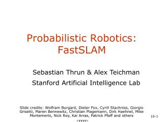
1. Probabilistic Robotics: FastSLAM Sebastian Thrun & Alex Teichman Stanford Artificial Intelligence Lab Slide credits: Wolfram Burgard, Dieter Fox, Cyrill Stachniss, Giorgio Grisetti, Maren Bennewitz, Christian Plagemann, Dirk Haehnel, Mike Montemerlo, Nick Roy, Kai Arras, Patrick Pfaff and others

2. The SLAM Problem • SLAM stands for simultaneous localization and mapping • The task of building a map while estimating the pose of the robot relative to this map • Why is SLAM hard?Chicken-or-egg problem: • a map is needed to localize the robot and a pose estimate is needed to build a map

3. The SLAM Problem A robot moving though an unknown, static environment Given: • The robot’s controls • Observations of nearby features Estimate: • Map of features • Path of the robot

4. Map Representations Typical models are: • Feature maps • Grid maps (occupancy or reflection probability maps)

5. Particle Filters • Represent belief by random samples • Estimation of non-Gaussian, nonlinear processes • Sampling Importance Resampling (SIR) principle • Draw the new generation of particles • Assign an importance weight to each particle • Resampling • Typical application scenarios are tracking, localization, …

6. Localization vs. SLAM • A particle filter can be used to solve both problems • Localization: state space < x, y, > • SLAM: state space < x, y, , map> • for landmark maps = < l1, l2, …, lm> • for grid maps = < c11, c12, …, c1n, c21, …, cnm> • Problem 1: The number of particles needed to represent a posterior grows exponentially with the dimension of the state space! • Problem 2: One of these particles has to “guess” the right map from the beginning

7. Dependencies • Is there a dependency between the dimensions of the state space? • If so, can we use the dependency to solve the problem more efficiently?

8. Dependencies • Is there a dependency between the dimensions of the state space? • If so, can we use the dependency to solve the problem more efficiently? • In the SLAM context • The map depends on the poses of the robot. • We know how to build a map given the position of the sensor is known.

9. Mapping using Landmarks l1 Landmark 1 z1 z3 observations . . . x1 x2 x3 xt x0 Robot poses u1 ut-1 u1 u0 controls z2 zt l2 Landmark 2 Knowledge of the robot’s true path renders landmark positions conditionally independent

10. Factored Posterior (Landmarks) poses map observations & movements Factorization first introduced by Murphy in 1999

11. Factored Posterior (Landmarks) poses map observations & movements SLAM posterior Robot path posterior landmark positions Does this help to solve the problem? Factorization first introduced by Murphy in 1999

12. Factored Posterior Robot path posterior(localization problem) Conditionally independent landmark positions

13. Rao-Blackwellization • This factorization is also called Rao-Blackwellization • Given that the second term can be computed efficiently, particle filtering becomes possible!

14. x, y,  Landmark 1 Landmark 2 Landmark M … FastSLAM • Rao-Blackwellized particle filtering based on landmarks [Montemerlo et al., 2002] • Each landmark is represented by a 2x2 Extended Kalman Filter (EKF) • Each particle therefore has to maintain M EKFs Particle #1 x, y,  Landmark 1 Landmark 2 Landmark M … Particle #2 x, y,  Landmark 1 Landmark 2 Landmark M … … Particle N

15. FastSLAM – Action Update Landmark #1 Filter Particle #1 Landmark #2 Filter Particle #2 Particle #3

16. FastSLAM – Sensor Update Landmark #1 Filter Particle #1 Landmark #2 Filter Particle #2 Particle #3

17. Weight = 0.8 Weight = 0.4 Weight = 0.1 FastSLAM – Sensor Update Particle #1 Particle #2 Particle #3

18. FastSLAM - Video

19. FastSLAM Complexity • Update robot particles based on control ut-1 • Incorporate observation zt into Kalman filters • Resample particle set N = Number of particles M = Number of map features

20. O(N) Constant time per particle O(N•log(M)) Log time per particle O(N•log(M)) Log time per particle O(N•log(M)) Log time per particle FastSLAM Complexity • Update robot particles based on control ut-1 • Incorporate observation zt into Kalman filters • Resample particle set N = Number of particles M = Number of map features

21. k  4 ? T F k  2 ? k  6 ? T F T F k  1 ? k  3 ? k  5 ? k  7 ? T F T F T F T F [m] [m] [m] [m] [m] [m] [m] [m] [m] [m] [m] [m] [m] [m] [m] [m] m1,S1 m2,S2 m3,S3 m4,S4 m5,S5 m6,S6 m7,S7 m8,S8 Log(M) Algorithm Represent particle as tree of Kalman Filters

22. k  4 ? T new particle F k  2 ? F T k  3 ? T F [m] [m] m3,S3 k  4 ? k  4 ? T T F F old particle k  2 ? k  2 ? k  6 ? k  6 ? T T F F T T F F k  1 ? k  1 ? k  3 ? k  3 ? k  1 ? k  1 ? k  3 ? k  3 ? T T F F T T F F T T F F T T F F [m] [m] [m] [m] [m] [m] [m] [m] [m] [m] [m] [m] [m] [m] [m] [m] [m] [m] [m] [m] [m] [m] [m] [m] [m] [m] [m] [m] [m] [m] [m] [m] m1,S1 m1,S1 m2,S2 m2,S2 m3,S3 m3,S3 m4,S4 m4,S4 m5,S5 m5,S5 m6,S6 m6,S6 m7,S7 m7,S7 m8,S8 m8,S8 Log(M) Algorithm Only update branches that change during resampling phase

23. O(N2) O(logN) The importance of scaling

24. Data Association Problem • A robust SLAM must consider possible data associations • Potential data associations depend also on the pose of the robot • Which observation belongs to which landmark?

25. Multi-Hypothesis Data Association • Data association is done on a per-particle basis • Robot pose error is factored out of data association decisions

26. Per-Particle Data Association Was the observation generated by the red or the blue landmark? P(observation|red) = 0.3 P(observation|blue) = 0.7 • Two options for per-particle data association • Pick the most probable match • Pick an random association weighted by the observation likelihoods • If the probability is too low, generate a new landmark

27. Results – Victoria Park • 4 km traverse • < 5 m RMS position error • 100 particles Blue = GPS Yellow = FastSLAM Dataset courtesy of University of Sydney

28. Results – Victoria Park (Video) Dataset courtesy of University of Sydney

29. Results – Data Association

30. FastSLAM Accuracy

31. Kalman Filter Kalman Filter Kalman Filter Kalman Filter 250 particles 250 particles 250 particles 100 particles 100 particles error 2 particles steps A funny finding (doesn’t generalize)

32. FastSLAM with Grid Maps Idea: Replace EKF Landmark map with occupancy grid map Q: Is this valid?

33. Mapping Abandoned Coal Mines

34. Mapping Abandoned Coal Mines

35. Particles in Mine Mapping

37. The Importance of Particle without particles with particles raw data

38. FastSLAM with Grid Maps map of particle 2 map of particle 1 map of particle 3 3 particles

39. Quality of 2D Maps 112 m

40. Outdoor Campus Map • 30 particles • 250x250m2 • 1.75 km (odometry) • 20cm resolution during scan matching • 30cm resolution in final map • 30 particles • 250x250m2 • 1.75 km (odometry) • 20cm resolution during scan matching • 30cm resolution in final map

41. FastSLAM Summary • FastSLAM factors the SLAM posterior into low-dimensional estimation problems • Scales to problems with over 1 million features • FastSLAM factors robot pose uncertainty out of the data association problem • Robust to significant ambiguity in data association • Allows data association decisions to be delayed until unambiguous evidence is collected • Advantages compared to the classical EKF approach • Update Complexity of O(N logM)