Download
1 / 13
720 likes | 2.64k Views
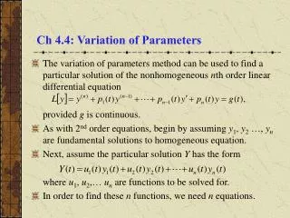
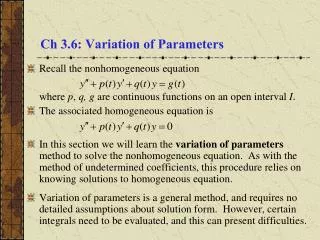
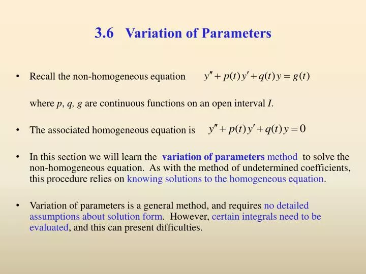
3.6 Variation of Parameters. Recall the non-homogeneous equation where p , q, g are continuous functions on an open interval I . The associated homogeneous equation is

E N D
3.6 Variation of Parameters • Recall thenon-homogeneous equation where p, q,g are continuous functions on an open interval I. • The associated homogeneous equation is • In this section we will learn the variation of parameters method to solve the non-homogeneous equation. As with the method of undetermined coefficients, this procedure relies on knowing solutions to the homogeneous equation. • Variation of parameters is a general method, and requires no detailed assumptions about solution form. However, certain integrals need to be evaluated, and this can present difficulties.
(Example 1) Consider (1) Find a general solution (common solution) of the homogeneous equation. • Find a particular solution of the nonhomogeneous equation by using the method of variation of parameters:
(Example 2) Consider (1) Find a general solution (common solution) of the homogeneous equation. (2) Find a particular solution of the nonhomogeneous equation.
(Example 3) Consider (1) Find a general solution (common solution) of the homogeneous equation. (2) Find a particular solution of the nonhomogeneous equation.
Example 1: Variation of Parameters (1 of 6) • We seek a particular solution to the equation below. • We cannot use the undetermined coefficients method since g(t) is a quotient of sin(t) or cos(t), instead of a sum or product. • Recall that the solution to the homogeneous equation is • To find a particular solution to the non-homogeneous equation, we begin with the form • Then • or
Example 1: Derivatives, 2nd Equation (2 of 6) • From the previous slide, • Note that we need two equations to solve for u1 and u2. The first equation is the differential equation. To get a second equation, we will require • Then • Next,
Example 1: Two Equations (3 of 6) • Recall that our differential equation is • Substituting y'' and y into this equation, we obtain • This equation simplifies to • Thus, to solve for u1 and u2, we have the two equations:
Example 1: Solve for u1'(4 of 6) • To find u1 and u2 , we first need to solve for • From second equation, • Substituting this into the first equation,
Example 1: Solve for u1 and u2(5 of 6) • From the previous slide, • Then • Thus
Example 1: General Solution (6 of 6) • Recall our equation and homogeneous solution yC: • Using the expressions for u1 and u2 on the previous slide, the general solution to the differential equation is
Summary • Suppose y1, y2 are fundamental solutions to the homogeneous equation associated with the nonhomogeneous equation above, where we note that the coefficient on y'' is 1. • To find u1 and u2, we need to solve the equations • Doing so, and using the Wronskian, we obtain • Thus
Theorem 3.6.1 • Consider the equations • If the functions p, q and g are continuous on an open interval I, and if y1 and y2 are fundamental solutions to Eq. (2), then a particular solution of Eq. (1) is and the general solution is