Download
1 / 36
360 likes | 436 Views
K - + Scattering from D Decays. Brian Meadows University of Cincinnati. {12}. {23}. {13}. 1. 1. 1. 2. 2. 2. 3. 3. 3. 1. 3. “Traditional” Dalitz Plot Analysis.

E N D
K-+ Scattering from D Decays Brian Meadows University of Cincinnati
{12} {23} {13} 1 1 1 2 2 2 3 3 3 1 3 “Traditional” Dalitz Plot Analysis • The “isobar model”, with relativistic Breit-Wigner (RBW) resonant terms, is widely used in studying 3-body decays of heavy quark mesons. • Amplitude for channel {ij}: • Each resonance “R” (mass MR, width R) assumed to have form NR 2 NRConstant R form factor D form factor spin factor
Traditional E791 DD+!KK-p+p+ ~138 % c2/d.o.f. = 2.7 Flat “NR” term does not give good description of data. Phys.Rev.Lett.89:121801,2002
“Traditional” Model for S-wave - E791 ~89 % c2/d.o.f. = 0.73 (95 %) Probability Mk = 797 § 19 § 42 MeV/c2 Gk = 410 § 43 § 85 MeV/c2 E. Aitala, et al, PRL 89 121801 (2002)
E791 (WMD) “Model-Independent”Partial-Wave Analysis (MIPWA) • Make partial-wave expansion of decay amplitude in angular momentum of K-+ system produced D form-factor • “Partial Wave:” • Describes invariant mass dependence of K-+ system • -> Related to K-+ • scattering ML(p,q) Watson Theorem holds that, up to elastic limit (K’ threshold for S-wave) K phases same as for elastic scattering.
Watson Theorem • The process P + c can be thought of as Borrowed from M. Pennington (hep-ph/0608016) • The only channel open below elastic limit is elastic scattering, so phase is same as for elastic scattering. • BUT the interaction between c and P introduces overall phase This might also depend on energy, in which case Watson theorem will not apply. FD FR means on mass shell.
MIPWA • Define S–wave amplitude at discrete points sK=sj. Interpolate elsewhere. model-independent - two parameters (ccj, j) per point • P- and D-waves are defined by known K* resonances and act as analyzers for the S-wave.
MIPWA • Phases are relative to K*(890) resonance. • Un-binned maximum likelihood fit: • Use 40 (cj, j) points for S • Float complex coefficients of KK*(1680) and K2*(1430) resonances • 4 parameters (d1680, 1680) and (d1430, 1430) ! 40 x 2 + 4 = 84 free parameters.
MIPWA – E791 Mass Distributions E791 15,079 signal events 94% purity 2/NDF = 272/277 (48%) S Phys.Rev.D73:032004,2006
Phases for S-, P- and D-waves are compared with measurements from LASS. S-wave phase S for E791 is shifted by -750 wrt LASS fs energy dependence differs below 1100 MeV/c2. P-wave phase does not match very well above K*(892) Probably artifact of model used Lower arrow is at threshold Upper arrow is at effective limit of elastic scattering observed by LASS. Watson Theorem - a direct test ? Elastic limit Kh’ threshold S P K1*(1410) D
A good fit was also made by constraining the shape of the S-wave phase to agree with that from K-+ scattering However: S-wave phase S for E791 still shifted by -750 wrt LASS fP match is even worse above K*(892) fD phase also shifts. Watson Theorem Enforced for S-wave S Elastic limit Kh’ threshold (1454 MeV/c2) P D
The BaBar Sample of D+K-++ • Skim carried out byRolf Andreassen. • A likelihood is based on PDFS (signal - MC) and PDFB (background - data sidebands) for each of the following quantities: • SignedD+ decay length l/sl • c2 probability for vertex • PLAB for D+ • Likelihood is product: Skim all with L>2
Rolf Andreassen’s Skim • K-p+p+ invariant mass vs. likelihood (L) (NOTE log scale). • Some purities:
D+ K-++ Dalitz Plot • Plot includes 500K events • of which 13K are background. • Obviously large S-wave content Interferes with K*(890) (and anything else in P-wave). • Some D-wave also present
Max. Likelihood Fit • Likelihood function covers 3-dimensions: • sK1, sK2 and also the reconstructed 3-body mass MK • Factorize MK dependence: • All events used in signal as well as sidebands have a D+ mass constraint. • Makes it possible to overlay Dalitz plot for sideband data directly on signal • Greatly simplifies computation of efficiency. • is efficiency Subscript s is signal Subscript b is background
Background Model • K-p+p+ invariant mass distribution from sample with L > 3 • Dalitz plot distributions in lower side-band, signal region and upper side-band (log. Scale) • Used directly as input to background function. PDF1b - bin-by-bin interpolation
Second Background • Probable origin • PDF2b = g(MK) x Gauss (M2K) Lost
Efficiency • Efficiency (%) over the Dalitz plot for various laboratory momentum ranges.
Efficiency vs. pLAB • Efficiency (%) vs laboratory momentum. • Lab. momentum for Data (black). • Lab. momentum for reconstructed, signal MC (red). No need to use efficiency as function of pLAB
“Traditional” Model for S-wave - BaBar 2/NDF = 20.1x10³ / 15.6x10³ - a very poor fit
Partial Waves from Model Fit Phase Magnitude NOTE – no K*(1410) Width of lines represents 1
E791 S-Wave Fit (on BaBar data) • S-wave is spline with 30 equally spaced points • P-wave is as in model fit, with complex coefficients floated. • D-wave also as in model fit – complex coefficient floated.
E791 S-Wave Fit (on BaBar data) 2/NDF = 1007/574 – better, but still a poor fit
The P-wave Problem • Problem is – the S-wave solution depends on assumptions made about the reference P-wave. • Models: • Add K1*(1410) RBW - this crowds the wave - SHOWN HERE • Could use K-matrix to avoid this – TO BE TRIED • Use LASS phases up to elastic limit (~110 MeV/c2) – TO BE TRIED BUT these all just transfer the ignorance. • Parametrize as table of complex values (spline) as for S-wave: • Sn(s) = splinen(s) - spline defined by n points. • Pm(s) = RBW[K*(890)] x splinem(s) • Not much progress on this yet. Uniqueness problem ? – can it be done at all?
Add K*(1410) to P-wave - BaBar 2/NDF = 18.8x10³ / 15.5x10³ – Better, but still a very poor fit
Spline for P-wave - Fit Procedures • Make E791 fit • Sn(s) from a table of n points. • Fix S-wave and fit P-wave same way • Pm(s) from a table of n points. • Fix P-wave and re-fit S-wave • Repeat cycle several times • SIMPLEX • Errors from likelihood scan • Alternatives • Cycle Magnitudes (both waves) and phases (both waves). • Use Binned likelihood – WORKS WELL • 2 fit. – WORKS LESS WELL Antimo’s procedure
|S| S phase S P phase |P| P Antimo’s Result
Some MC Tests • Generate toy MC corresponding to model fit to data • No background • Look for self-consistency between fit and generated quantities
Kappa Model Test Output Input
MC Test – S-wave Only • S-wave is fitted tospline with 40 equally spaced points • P-wave is fixed as in model fit (but defined as a spline). • D-wave complex coefficient floated.
MC Test – P-wave Only • S-wave is fixed as in model fit. • P-wave is fitted tospline with 40 equally spaced points • D-wave complex coefficient floated.
MC Test – Migrad S-P Cycles Cycling does work, but convergence seems far away even after 16 cycles! S -2lnL P S etc # Function Calls
Mag -2lnL Phase Mag etc # Function Calls MC Test –Magn./Phase Cycles Cycling does work, but convergence seems far away even after 16 cycles!
BUT – Float S- and P-waves Together !! Maybe it is not possible tofindboth S- and P-wave amplitudes without a definite form for one of them.
MIPWA for Both S- and P-waves? • Regions exist where the P-wave is much smaller than the S-wave This makes phase measurements more difficult to make
Summary • So far, we have gone as far as E791 did, but the next steps need some more work. • We conclude that the S-wave can be well determined if the P-wave is known • Understanding the P-wave is a challenging problem. • New ideas how to parametrize the P-wave need be considered.