Download
1 / 17
170 likes | 176 Views
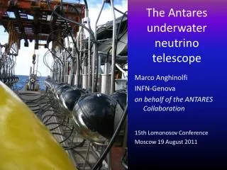
Positioning system of the ANTARES Neutrino Telescope. Miguel Ardid (IGIC –UPV) on behalf of the ANTARES Collaboration. VLVNT’08 – Toulon - April 2008. Contents. ANTARES Detector Motivation and Basics for the Positioning system Line Shape Model: Mechanics Input and Output

E N D
Positioningsystem of theANTARES Neutrino Telescope Miguel Ardid (IGIC –UPV) on behalf of the ANTARES Collaboration VLVNT’08 – Toulon - April 2008
Contents • ANTARES Detector • Motivation and Basics for the Positioning system • Line Shape Model: • Mechanics • Input and Output • Instrumentation: • Compass-Tilmeter System • Acoustic Sytem • Complementary Oceanography • Results: • Acoustic Examples • Comparison Line Model – Acoustics • Comparison Line Model – ADCP • Conclusions
ANTARES Detector (reminder) 2500m 450 m ~70 m • 900 PMTs • 12 lines • 25 storeys / line • 3 PMTs / storey 40 km to shore 10 lines + IL deployed, connected and taking data M. Circella’s talk Status of the ANTARES underwater neutrino telescope Junction Box Interlink cables
Motivation and Basics for the Positioning System • A positioning system for the optical modules (OMs) is needed: • Sea currents result on drifts of the top of the strings (and OMs) by several meters • However, muon track reconstruction is based on: • precise arrival time of Cherenkov photons to the optical modules (~1 ns) • knowledge of the OM position with the corresponding resolution (~20 cm) • ANTARES has a positioning system to monitor the position of the OMs continuously. It is based in the reconstruction of the shape of the line from the information of: • High frequency long baseline (LBL) acoustic system: • Gives the positions of few hydrophones in the line • Tiltmeters and Compasses: • giving the local tilt and heading angles of each storey with optical modules • plus oceanography instrumentation: • to determine the sound velocity in sea water and the sea current
Line Shape Model. Mechanics Inclination of line results from buoyancy P and horizontal force F due to sea current: height in m z N N tanF /P j j P i i r j=i j=i zenith angle i P = buoyancy – weight F = 1/2 cw A v j sea current v F i 2 j j j of element j of the line tandr/dz i integration Line shape: displacement in m r(z) = a v z - b v ln[1-cz] 2 2 the only unknown is sea current velocity V (Vx, Vy) a, b, c known mechanical constants Cwj: drag coef. determined by hydrodyn. study of the storey in Ifremer pool
Line Shape Model. Inputs and Outputs • Input: • Positions from hydrophones (5 points along the line) • Tilts and Heading from Compass/Tiltmeter (in each storey, 25 gradients) • Geometrical Constants (cable length, storey parameters etc.) • Output: • Positions of allStoreys • Storey orientation • Sea currentvelocity (fromthefit)
Instrumentation. Compass-Tilmeter System • Integration of Tiltmeter-Compass sensor board in ANTARES electronic containers: • Local measurement of tilts (roll, pitch) and heading of storeys • Selected sensor TCM2 by NPI.: • Integrated on a more general instrumental board • RS232 serial link interface, low power consumption (20 mA) • Measurement range : ±20° on 2 tilt axes, 360º on heading • Accuracy : 0.2° in tilt, 1.0° in heading • Compensation of parasitic magnetic fields • Performance, linearity checked at CPPM (good agreement with spec. )
Instrumentation. Acoustic System • Positioningisdeterminedusingacoustictriangulationbetweenfixedemittersonthe sea floor and hydrophonesonthelines • Distances are obtainedfromthetravel timemeasurement of theacoustic wave. • HF-LBL system characteristics: • Frequency range (40 – 60 kHz) • 5 hydrophones per line, (S1, S8, S14, S20, S25) • A transmitter/receiver per line at the BSS (line bottom) + autonomoustransponders • Electronicboardsforsettings, emission, detection, filtering and recording • Full detector positioningobtainedevery 1-2minutes
Instrumentation. Complementary Oceanography • Pressure sensor: • Givesthedepth of each line bottom • Precision: ±0.01 bar (~ 0.1 m) • CTD probe : • Conductivity, temperature, depthusedto compute soundvelocity • Precisions : (±0.01mS/cm, ±0.01 °C, ±0.01 bar) • SoundVelocimeter: • directmeasurement of soundvelocityon a 20 cm basis • Precision: ±0.05 m/s • AcousticDopplerCurrentProfilers (ADCP): • measurement of the sea currentvelocity • Precision: ± 1 cm/s Sound velocity (m/s)
Results. Acoustic examples • Examples of variation of the vertical distance between the emitter and top receiver on Line 5 compared to sea current:
Results. Acoustic examples • Examples of altitude variation on bottom & top Storeys of Line 4 • As expected, altitudes show good correlation with higher amplitude variation on top storeys
Results. Acoustic examples • Examples of radial displacement on 5 Line 4 hydrophones given by triangulation • Origin of the reference frame is the line axis • Typically displacement of the line top storeys is of few metres • New acoustic data are obtained every minute
Results. Acoustic examples • Examples of radial displacement on Line 4 hydrophones given by triangulation • Hydrophone displacements followed with few cm accuracy • Larger displacements are observed for the top storeys • Line movement dominated by East-West heading of the Ligurian current.
Measurements and Results. • Examples showing the similar behaviour in the different lines
Results. Comparison Line Model - Acoustics • Comparison between hydrophone positions given by Line model and by acoustic triangulation (Feb – June 2007) Blue: alignment (no acoustic input) Green: alignment (with acoustic input) Red: acoustic triangulation Hydrophone position Line Model vs. Acoustic directly Line 1 Bottom floor Y (m) 14 m RMS = 3 cm 15 days DY (m) Hydrophone position Line Model vs. Acoustic directly Line 1 Top floor Y (m) RMS = 7cm 14 m DY (m) 18 m X (m)
Results. Comparison Line Model - ADCP Red: from ADCP Green: from Model (Line 1 fit)) Sea Current Velocity (m/s)
Conclusions • The positioning system (acoustics + tiltmeters) for the 10 lines in operation is functional and within specifications • The required spatial reconstruction of 20 cm per OM is achieved • The use of independent systems allows cross-checks and to detect and solve possible systematic uncertainties • Due to the good performance and flexibility of the positioning system, it provides a good starting point for the design of the positioning calibration system of a cubic kilometre neutrino telescope. Thank you for the attention