Download
1 / 18
190 likes | 550 Views
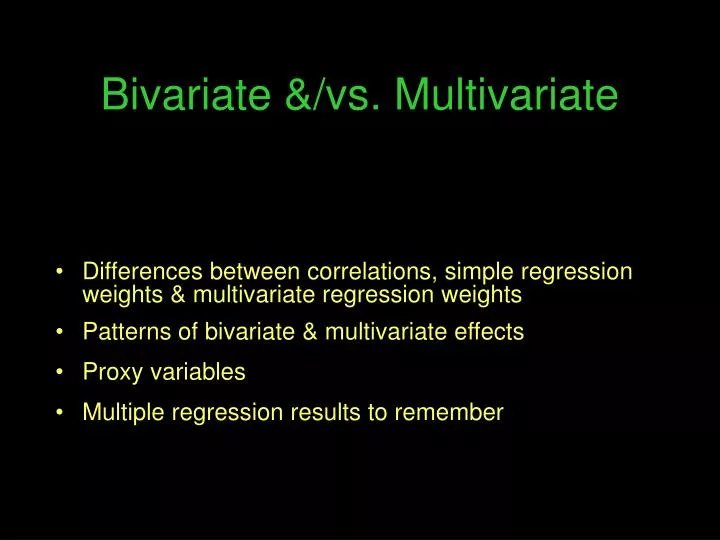
Bivariate &/vs. Multivariate . Differences between correlations, simple regression weights & multivariate regression weights Patterns of bivariate & multivariate effects Proxy variables Multiple regression results to remember.

E N D
Bivariate &/vs. Multivariate • Differences between correlations, simple regression weights & multivariate regression weights • Patterns of bivariate & multivariate effects • Proxy variables • Multiple regression results to remember
It is important to discriminate among the information obtained from ... • a simple correlation • tells the direction and strength of the linear relationship between two quantitative/binary variables • a regression weight from a simple regression • tells the expected change (direction and amount) in the criterion for a 1-unit change in the predictor • a regression weight from a multiple regression model • tells the expected change (direction and amount) in the criterion for a 1-unit change in that predictor, holding the value of all the other predictors constant
Correlation r For aquantitative predictor sign of r = the expected direction of change in Y as X increases size of r = is related to the strength of that expectation For abinary x with 0-1 coding sign of r= tells which coded group X has higher mean Y size of r= is related to the size of that group Y mean difference
Simple regression y’ = bx + a raw score form b -- raw score regression slope or coefficient a-- regression constant or y-intercept For aquantitative predictor a = the expected value of y if x = 0 b = the expected direction and amount of change in the criterion for a 1-unit increase in the For abinary x with 0-1 coding a= the mean of y for the group with the code value = 0 b= the mean y difference between the two coded groups
raw score regressiony’ = b1x1 + b2x2 + b3x3 + a • each b • represents the unique and independent contribution of that predictor to the model • for a quantitative predictor tells the expected direction and amount of change in the criterion for a 1-unit change in that predictor, while holding the value of all the other predictors constant • for a binary predictor (with unit coding -- 0,1 or 1,2, etc.), tells direction and amount of group mean difference on the criterion variable, while holding the value of all the other predictors constant • a • the expected value of the criterion if all predictors have a value of 0
What influences the size of r, b & r -- bivariate correlation range = -1.00 to +1.00 -- strength of relationship with the criterion -- sampling “problems” (e.g., range restriction) b (raw-score regression weights range = -∞ to ∞-- strength of relationship with the criterion -- collinearity with the other predictors -- differences between scale of predictor and criterion -- sampling “problems” (e.g., range restriction) -- standardized regression weights range = -1.00 to +1.00-- strength of relationship with the criterion -- collinearity with the other predictors -- sampling “problems” (e.g., range restriction) Difficulties of determining “more important contributors” -- b is not very helpful - scale differences produce b differences -- works better, but limited by sampling variability and measurement influences (range restriction) Only interpret “very large” differences as evidence that one predictor is “more important” than another
Venn diagrams representing r & b ry,x2 ry,x1 x2 x3 x1 ry,x3 y
Remember that the b of each predictor represents the part of that predictor shared with the criterion that is not shared with any other predictor -- the unique contribution of that predictor to the model bx2 bx1 x2 x3 x1 bx3 y
Important Stuff !!! There are two different reasons that a predictor might not be contributing to a multiple regression model... • the variable isn’t correlated with the criterion • the variable is correlated with the criterion, but is collinear with one or more other predictors, and so, has no independent contribution to the multiple regression model x1 y x3 x2 X1 has a substantial r with the criterion and has a substantial b x2 has a substantial r with the criterion but has a small b because it is collinear with x1 x3 has neither a substantial r nor substantial b
We perform both bivariate (correlation) and multivariate (multiple regression) analyses – because they tell us different things about the relationship between the predictors and the criterion… Correlations (and bivariate regression weights) tell us about the “separate” relationships of each predictor with the criterion (ignoring the other predictors) Multiple regression weights tell us about the relationship between each predictor and the criterion that is unique or independent from the other predictors in the model. Bivariate and multivariate results for a given predictor don’t always agree – but there is a small number of distinct patterns…
There are 5 patterns of bivariate/multivariate relationship Simple correlation with the criterion - 0 + “Suppressor effect” – bivariate relationship & multivariate contribution (to this model) have different signs Bivariate relationship and multivariate contribution (to this model) have same sign “Suppressor effect” – no bivariate relationship but contributes (to this model) Multiple regression weight + 0 - Non-contributing – probably because colinearity with one or more other predictors Non-contributing – probably because of weak relationship with the criterion Non-contributing – probably because colinearity with one or more other predictors Bivariate relationship and multivariate contribution (to this model) have same sign “Suppressor effect” – bivariate relationship & multivariate contribution (to this model) have different signs “Suppressor effect” – no bivariate relationship but contributes (to this model)
Bivariate & Multivariate contributions – DV = Grad GPA predictor age UGPA GRE work hrs #credits r(p) .11(.32) .45(.01) .38(.03) -.21(.06) .28(.04) b(p) .06(.67) 1.01(.02) .002(.22) .023(.01) -.15(.03) UGPA Bivariate relationship and multivariate contribution (to this model) have same sign “Suppressor variable” – no bivariate relationship but contributes (to this model) “Suppressor variable” – bivariate relationship & multivariate contribution (to this model) have different signs Non-contributing – probably because colinearity with one or more other predictors Non-contributing – probably because of weak relationship with the criterion work hrs #credits GRE age
Bivariate & Multivariate contributions – DV = Pet Quality predictor #fish #reptiles ft2 #employees #owners r(p) -.10(.31) .48(.01) -.28(.04) .37(.03) -.08(.54) b(p) -.96(.03) 1.61(.42) 1.02(.02) 1.823(.01) -.65(.83) #fish #reptiles ft2 #employees #owners “Suppressor variable” – no bivariate relationship but contributes (to this model) Non-contributing – probably because of colinearity with one or more other predictors “Suppressor variable” – bivariate relationship & multivariate contribution (to this model) have different signs Bivariate relationship and multivariate contribution (to this model) have same sign Non-contributing – probably because of weak relationship with the criterion
Proxy variables • Remember (again) we are not going to have experimental data! • The variables we have might be the actual causal variables influencing this criterion, or (more likely) they might only be correlates of those causal variables – proxy variables • Many of the “subject variables” that are very common in multivariate modeling are of this ilk… • is it really “sex,” “ethnicity”, “age” that are driving the criterion – or is it all the differences in the experiences, opportunities, or other correlates of these variables? • is it really the “number of practices” or the things that, in turn, produced the number of practices that were chosen? Again, replication and convergence (trying alternative measure of the involved constructs) can help decide if our predictors are representing what we think the do!!
Proxy variables In sense, proxy variables are a kind of “confounds” because we are attributing an effect to one variable when it might be due to another. We can take a similar effect to understanding proxys that we do to understanding confounds we have to rule out specific alternative explanations !!! An example r gender, performance = .4 Is it really gender? Motivation, amount of preparation & testing comfort are some variables that have gender differences and are related to perf. So, we run a multiple regression with all four as predictors. If gender doesn’t contribute, then it isn’t gender but the other variables. If gender contributes to that model, then we know that “gender” in the model is “the part of gender that isn’t motivation, preparation or comfort” but we don’t know what it really is….
As we talked about last time, collinearity among the multiple predictors can produce several patterns of bivariate-multivariate contribution. There are three specific combinations you should be aware of (all of which are fairly rare, but can be perplexing if they aren’t expected)… • Multivariate Power -- sometimes a set of predictors none of which are significantly correlated with the criterion can be produce a significant multivariate model (with one or more contributing predictors) • How’s that happen? • The error term for the multiple regression model and the test of each predictor’s b is related to 1-R2 of the model • Adding predictors will increase the R2 and so lower the error term – sometimes leading to the model and 1 or more predictors being “significant” • This happens most often when one or more predictors have “substantial” correlations, but the sample power is low
Null Washout -- sometimes a set of predictors with only one or two significant correlations to the criterion will produce a model that is not significant. Even worse, those significantly correlated predictors may or may not be significant contributors to the non-significant model • How’s that happen? • The F-test of the model R2 really (mathematically) tests the average contribution of all the predictors in the model • So, a model dominated by predictors that are not substantially correlated with the criterion might not have a large enough “average” contribution to be statistically significant • This happens most often when the sample power is low and there are many predictors R² / k F = --------------------------------- (1 - R²) / (N - k - 1)
Extreme collinearity -- sometimes a set of predictors all of which are significantly correlated with the criterion can be produce a significant multivariate model with one or more contributing predictors • How’s that happen? • Remember that in a multiple regression model each predictors b weight reflects the unique contribution of that predictor in that model • If the predictors are all correlated with the criterion but are more highly correlated with each other, each of their “overlap” with the criterion is shared with 1 or more other predictors and no predictor has much unique contribution to that very successful (high R2) model x1 x2 x3 x4 y