Download

1 / 44
450 likes | 623 Views
Statistics for Microarrays. Normalization. Class web site: http://statwww.epfl.ch/davison/teaching/Microarrays/ETHZ/. Biological question Differentially expressed genes Sample class prediction etc. Experimental design. Microarray experiment. 16-bit TIFF files. Image analysis.

E N D
Statistics for Microarrays Normalization Class web site: http://statwww.epfl.ch/davison/teaching/Microarrays/ETHZ/
Biological question Differentially expressed genes Sample class prediction etc. Experimental design Microarray experiment 16-bit TIFF files Image analysis (Rfg, Rbg), (Gfg, Gbg) Normalization R, G Estimation Testing Clustering Discrimination Biological verification and interpretation
Preprocessing: Data Visualization • Was the experiment a success? • Are there any specific problems? • What analysis tools should be used?
Tools for Microarray Normalization and Analysis • Both commercial and free software • R (use sma package or Bioconductor: http://www.bioconductor.org/)
Red/Green overlay images Co-registration and overlay offers a quick visualization, revealing information on color balance, uniformity of hybridization, spot uniformity, background, and artefacts such as dust or scratches Bad: high bg, ghost spots, little d.e. Good: low bg, detectable d.e.
Scatterplots: always log*, always rotate log2R vs log2G M=log2R/G vs A=log2√RG * Other transformations can provide improvement
Histograms Signal/Noise = log2(spot intensity/background intensity)
Boxplots of log2R/G Liver samples from 16 mice: 8 WT, 8 ApoAI KO
Highlighting extreme log ratios Top (black) and bottom (green) 5% of log ratios
Pin group (sub-array) effects Lowess lines through points from pin groups Boxplots of log ratios by pin group
Boxplots and highlighting pin group effects Log-ratios Clear example of spatial bias Print-tip groups
Clearly visible plate effects KO #8 Probes: ~6,000 cDNAs, including 200 related to lipid metabolism. Arranged in a 4x4 array of 19x21 sub-arrays.
Time of printing effects spot number Green channel intensities (log2G). Printing over 4.5 days. The previous slide depicts a slide from this print run.
Preprocessing: Normalization • Why? To correct for systematic differences between samples on the same slide, or between slides, which do not represent true biological variation between samples • How do we know it is necessary? By examining self-self hybridizations, where no true differential expression is occurring. There are dye biases which vary with spot intensity, location on the array, plate origin, pins, scanning parameters,…
Self-self hybridizations False color overlay Boxplots within pin-groups Scatter (MA-)plots
Similar patterns apparent in non self-self hybridizations From the NCI60 data set (Stanford web site)
Normalization Methods (I) • Normalization based on a global adjustment log2 R/G -> log2 R/G - c = log2 R/(kG) Choices for k or c = log2k are c = median or mean of log ratios for a particular gene set (e.g. all genes, or control or housekeeping genes). Or, total intensity normalization, where k = ∑Ri/ ∑Gi. • Intensity-dependent normalization Here, run a line through the middle of the MA plot, shifting the M value of the pair (A,M) by c=c(A), i.e. log2 R/G -> log2 R/G - c (A) = log2 R/(k(A)G). One estimate of c(A) is made using the LOWESS function of Cleveland (1979): LOcally WEighted Scatterplot Smoothing.
Normalization Methods (II) • Within print-tip group normalization In addition to intensity-dependent variation in log ratios, spatial bias can also be a significant source of systematic error. Most normalization methods do not correct for spatial effects produced by hybridization artefacts or print-tip or plate effects during the construction of the microarrays. It is possible to correct for both print-tip and intensity-dependent bias by performing LOWESS fits to the data within print-tip groups, i.e. log2 R/G -> log2 R/G - ci(A) = log2 R/(ki(A)G), where ci(A) is the LOWESS fit to the MA-plot for the ith grid only.
Normalization: Which Spots to use? The LOWESS lines can be run through many different sets of points, and each strategy has its own implicit set of assumptions justifying its applicability. For example, the use of a global LOWESS approach can be justified by supposing that, when stratified by mRNA abundance, a) only a minority of genes are expected to be differentially expressed, or b) any differential expression is as likely to be up-regulation as down-regulation. Pin-group LOWESS requires stronger assumptions: that one of the above applies within each pin-group. The use of other sets of genes, e.g. control or housekeeping genes, involve similar assumptions.
Normalization makes a difference Global scale, global lowess, pin-group lowess; spatial plot after, smooth histograms of M after
Normalization by controls:Microarray Sample Pool titration series Pool the whole library Control set to aid intensity-dependent normalization Different concentrations in titration series Spotted evenly spread across the slide in eachpin-group
Comparison of Normalization Schemes(courtesy of Jason Goncalves) • No consensus on best normalization method • Experiment done to assess the common normalization methods • Based on reciprocal labeling experimental data for a series of 140 replicate experiments on two different arrays each with 19,200 spots
DESIGN OF RECIPROCAL LABELING EXPERIMENT • Replicate experiment with same mRNA pools but invert fluors (dye swap) • Replicates are independent experiments • Scan, quantify, normalize as usual
Scale normalization: between slides Boxplots of log ratios from 3 replicate self-self hybridizations Left panel: before normalization Middle panel: after within print-tip group normalization Right panel: after a further between-slide scale normalization
The “NCI 60” experiments (no bg) Some scale normalization seems desirable
Scale normalization: another data set Log-ratios • Only small differences in spread apparent; no action required. • `
One way of taking scale into account Assumption: All slides have the same spread in M True log ratio is mij where i represents differentslides and j represents different spots. Observed is Mij, where Mij = aimij Robust estimate of ai is MADi = medianj { |yij - median(yij) | }
A slightly harder normalization problem Global lowess doesn’t do the trick here
But not completely Still a lot of scatter in the middle in a WT vs KO comparison
Effects of previous normalization Before normalization After print-tip-group normalization
Within print-tip-group box plots of M after print-tip-group normalization
Taking scale into account, cont. Assumption: All print-tip-groups have the same spread in M True log ratio is mij where i represents different print-tip-groups and j represents different spots. Observed is Mij, where Mij = aimij Robust estimate of ai is MADi = medianj { |yij - median(yij) | }
Effect of location & scale normalization Clearly care is needed in making decisions like this
A comparison of three M v A plots Print-tip normalization Print tip & scale n Unnormalized
The same normalization on another data set Before . After
Normalization: Summary • Reduces systematic (not random) effects • Makes it possible to compare several arrays • Use logratios (M vs A plots) • Lowess normalization (dye bias) • MSP titration series – composite normalization • Pin-group location normalization • Pin-group scale normalization • Between slide scale normalization • Control Spots • Normalization introduces more variability • Outliers (bad spots) are handled with replication
Affymetrix Oligo Chips • Only one “color” • Different technology, different normalization issues • Affy chip normalization is an active research area – see http://www.stat.berkeley.edu/users/terry/zarray/Affy/affy_index.html
Pre-processed cDNA Gene Expression Data Slides On p genes for n slides: p is O(10,000), n is O(10-100), but growing, slide 1 slide 2 slide 3 slide 4 slide 5 … 1 0.46 0.30 0.80 1.51 0.90 ... 2 -0.10 0.49 0.24 0.06 0.46 ... 3 0.15 0.74 0.04 0.10 0.20 ... 4 -0.45 -1.03 -0.79 -0.56 -0.32 ... 5 -0.06 1.06 1.35 1.09 -1.09 ... Genes Gene expression level of gene 5 in slide 4 = (normalized) log2(Red / Green) These values are conventionally displayed on a red(>0)yellow (0)green (<0) scale.
Terry Speed (UCB and WEHI) Jean Yee Hwa Yang (UCB) Sandrine Dudoit (UCB) Ben Bolstad (UCB) Natalie Thorne (WEHI) Ingrid Lönnstedt (Uppsala) Henrik Bengtsson (Lund) Jason Goncalves (Iobion) Matt Callow (LLNL) Percy Luu (UCB) John Ngai (UCB) Vivian Peng (UCB) Dave Lin (Cornell) Acknowledgments