Download
1 / 79
890 likes | 1.29k Views
5-1 Continuous Random Variables 5-2 Standard Normal Distribution 5-3 Applications of Normal Distributions: Finding Probabilities Finding Values 5-4 Determining Normality 5-5 The Central Limit Theorem 5-6 Normal Distribution as Approximation to Binomial Distribution.

E N D
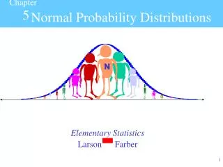
5-1 Continuous Random Variables 5-2 Standard Normal Distribution 5-3 Applications of Normal Distributions: Finding Probabilities Finding Values 5-4 Determining Normality 5-5 The Central Limit Theorem 5-6 Normal Distribution as Approximation to Binomial Distribution Chapter 5Normal Probability Distributions
Uniform (rectangular) distribution Normal distribution Standard Normal distribution Note: Continuous random variables are typically represented by curves Discrete random variables are typically represented by histograms 5-1 Continuous Random Variables
Density Curve (or probability density function) is the graph of a continuous probability distribution Definitions Properties 1. The total area under the curve must equal 1. 2. Every point on the curve must have a vertical height that is 0 or greater.
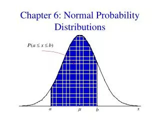
Two Important Points: • Because the total area under the density curve is equal to 1, there is a correspondence between area and probability. • To find probability in a continuous distribution just find the area under the curve(Calculus)
Rectangular Distribution Simplest type of continuous probability distribution random variable values are spread evenly over the range of possibilities; graph results in a rectangular shape. Finding probability is the same as finding the area of a rectangle Uniform Distribution
Using Area to Find Probability of Class Length Find P(51.5 < x < 52)
Uniform Distribution Formal definition of density function 1 Definitions y = for a < x < b b - a From previous example: a = 50 and b = 52 1 1 y = = 2 52 - 50
Let X be a uniform random variable, find the density function for each and graph If X is between 0 and 5 Find a. p(x > 4) b. p(1 < x < 5) If X is between 6 and 12 Find a. Find p(x > 6) b. p(x < 5) c. p(x > 12) Go to excel Examples:
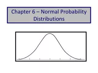
Continuous random variable Normal distribution Curve is bell shaped and symmetric µ Score Normal Distribution x - µ2 ( ) 1 2 y = e Formula 2 p
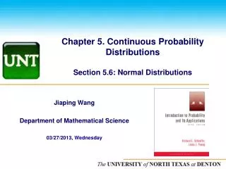
Standard Normal Distribution: a normal probability distribution that has a mean of 0 and a standard deviation of 1, and the total area under its density curve is equal to 1. Definition Area found in z - table or calculator 1 z2 2 y = e 2 p 0.4429 z = 1.58 0 Note: Typically ‘z’ denotes a standard normal random variable
P(a < z < b) denotes the probability that the z score is between a and b P(z > a) denotes the probability that the z score is greater than a P (z < a) denotes the probability that the z score is less than a Notation
Uses calculus to find the area under density function curve associated with a particular z-value Table available on website Calculator is easier Z - Table
the distance along horizontal scale of the standard normal distribution; refer to the leftmost column and top rowofTable Area the region under the curve; refer to the values in the body of Table To find:zScore
TI-83 Calculator Finding Areas of Standard Normal Distribution • Press 2nd Distr • Choose normcdf • Enter normcdf(low z value, high z value) • Press enter Note: if low z value is negative infinity use –E99 if high z value is positive infinity use E99
The probability that the chosen thermometer will measure freezing water less than 1.58 degrees is 0.9429. Example: If thermometers have an average (mean) reading of 0 degrees and a standard deviation of 1 degree for freezing water and if one thermometer is randomly selected, find the probability that, at the freezing point of water, the reading is less than 1.58 degrees. P (z < 1.58) = 0.9429
94.29% of the thermometers have readings less than 1.58 degrees. Example: If thermometers have an average (mean) reading of 0 degrees and a standard deviation of 1 degree for freezing water and if one thermometer is randomly selected, find the probability that, at the freezing point of water, the reading is less than 1.58 degrees. P (z < 1.58) = 0.9429
The probability that the chosen thermometer with a reading above –1.23 degrees is 0.8907. Example: If thermometers have an average (mean) reading of 0 degrees and a standard deviation of 1 degree for freezing water, and if one thermometer is randomly selected, find the probability that it reads (at the freezing point of water) above –1.23 degrees. P (z > –1.23) = 0.8907
89.07% of the thermometers have readings above –1.23 degrees. Example: If thermometers have an average (mean) reading of 0 degrees and a standard deviation of 1 degree for freezing water, and if one thermometer is randomly selected, find the probability that it reads (at the freezing point of water) above –1.23 degrees. P (z > –1.23) = 0.8907
The probability that the chosen thermometer has a reading between – 2.00 and 1.50 degrees is 0.9104. Example: Athermometer is randomly selected. Find the probability that it reads (at the freezing point of water) between –2.00 and 1.50 degrees. P (z < –2.00) = 0.0228 P (z < 1.50) = 0.9332 P (–2.00 < z < 1.50) = 0.9332 –0.0228 = 0.9104
If many thermometers are selected and tested at the freezing point of water, then 91.04% of them will read between –2.00 and 1.50 degrees. Example: Athermometer is randomly selected. Find the probability that it reads (at the freezing point of water) between –2.00 and 1.50 degrees. P (–2.00 < z < 1.50) = 0.9104
Let’s try several examples examples (sketch a graph) • P(Z < 1.45) • P(Z < -1.45) • P(Z > 1.45) • P(Z > -1.45) • P(0 < Z < 1.45) • P(-1.45 < Z < 0) • P(-1.45 < Z < 1.45) • P(-1.35 < Z < 1.45) • P(.56 < Z < 1.45) Test Problems
Frequently used Z – Scores • Z = 1.28 • Z = 1.645 • Z = 1.96 • Z = 2.33 • Z = 2.58 To illustrate why, find • P(Z > 1.28) • P(Z > 1.645) • P(Z > 1.96) • P(Z > 2.33) • P(Z > 2.58)
The Empirical Rule Standard Normal Distribution: µ = 0 and = 1 0.1% 99.7% of data are within 3 standard deviations of the mean 95% within 2 standard deviations 68% within 1 standard deviation 34% 34% 2.4% 2.4% 0.1% 13.5% 13.5% x - 3s x - 2s x - s x x+s x+2s x+3s
1. Draw a bell-shaped curve, draw the centerline, and identify the region under the curve that corresponds to the given probability. 2. Use the invNorm calculator function to determine the corresponding z score. Finding a z - score when given a probability (Area)
Finding z Scores when Given Probabilities Finding the 95th Percentile 95% 5% 5% or 0.05 0.45 0.50 1.645 0 invNorm(.95) (z score will be positive)
Finding z Scores when Given Probabilities Finding the 10th Percentile 90% 10% Bottom 10% 0.10 0.40 z 0 (zscore will be negative)
Finding z Scores when Given Probabilities Finding the 10th Percentile 90% 10% Bottom 10% 0.10 0.40 -1.28 0 invNorm(.10) (zscore will be negative)
Examples: • Find the Z score that corresponds the following percentiles • 50th • 25th • 75th • Find the Z score(s) for the following areas from the mean • 0.4495 • 0.3186
Find the Z score when given the probability (sketch each) • P(0 < z < a) = .34 • P(-b < z < b) = .8442 • P(z > c) = .056 • P(z > d) = .8844 • P(z < e) = .3400 • These are similar to HW #4 (Extra Credit)
x - µ z = 5-3 Applications of Normal Distributions If 0or 1 (or both), we will convert values to standard scores using the z-score formula we learned in Chapter 2, then procedures for working with all normal distributions are the same as those for the standard normal distribution. Note: z scores are real numbers that have no units
x– z = Converting to Standard Normal Distribution
= 36 =1.4 38.8 – 36.0 z = = 2.00 1.4 Probability of Sitting Heights Less Than 38.8 Inches
= 36 =1.4 Probability of Sitting Heights Less Than 38.8 Inches P ( x < 38.8 in.) = P(z < 2) normalcdf (-E99,2) = 0.9772
Probability of Weight between 150 pounds and 200 pounds 200 - 150 µ = 150 z = = 2.00 σ=25 25 x Weight 150200 z 0 2.00
Probability of Weight between 150 pounds and 200 pounds normalcdf (0,2) = .4772 µ = 150 σ=25 x Weight 150200 z 0 2.00
Probability of Weight between 150 pounds and 200 pounds There is a 0.4772 probability of randomly selecting a woman with a weight between 150 and 200 lbs. µ = 150 σ=25 x Weight 150200 z 0 2.00
Probability of Weight between 150 pounds and 200 pounds OR - 47.72% of women have weights between 150 lb and 200 lb. µ = 150 σ=25 x Weight 150200 z 0 2.00
Normal Distribution: Finding Values From Known Areas
Don’t confuse zscores and areas. Choose the correct (right/left) side of the graph. A z score must be negative whenever it is located to the left of the centerline of 0. Cautions to keep in mind
1. Sketch a normal distribution curve, enter the given probability or percentage in the appropriate region of the graph, and identify thexvalue(s) being sought. Find the z score invNorm(area) Make thez score negative if it is located to the left of the centerline. 3. Use x= µ + (z• )to find the value for x or invNorm(area,µ,σ) 4. Refer to the sketch of the curve to verify that the solution makes sense. Procedure for Finding Values Using TI-83 Calculator
Finding P10 for Weights of Women x = + (z ● ) x = 150 + (-1.28 • 25) = 118.75 µ = 150 σ=25 0.10 0.40 0.50 x Weight x = ? 150 z 0 -1.28
Finding P10 for Weights of Women The weight of 119 lb (rounded) separates the lowest 10% from the highest 90%. 0.10 0.40 0.50 x Weight x = 119 150 z 0 -1.28
In Class Example A tire company finds the lifespan for one brand of its tires is normally distributed with a mean of 48,500 miles and a standard deviation of 5000 miles. a) What is the probability that a randomly selected tire will be replaced in 40,000 miles or less? b) If the manufacturer is willing to replace no more than 10% of the tires, what should be the approximate number of miles for a warranty? Similar to hw #9 – Test problem
REMEMBER! Make the z score negative if the value is located to the left (below) the mean. Otherwise, the z score will be positive.
Extra Credit A teacher informs her statistics class that a test if very difficult, but the grades will be curved. Scores are normally distributed with a mean of 25 and standard deviation of 5. The grades will be curved according to the following scheme. A’s: Top 10% B’s: Between the top 10% and top 30%. C’s: Between the bottom 30% and top 30% D’s: Between the bottom 10% and bottom 30% F’s: Bottom 10% Find the numerical limits for each grade. Include sketch.
Determining Normality Use Descriptive Methods • Histogram • Dot Plot • Stem-leaf