Download
1 / 23
230 likes | 381 Views
Extreme Temperature Regimes during the Cool Season. Robert X. Black Rebecca Westby School of Earth and Atmospheric Sciences Georgia Institute of Technology, Atlanta, Georgia DOE/BER Regional and Global Climate Modeling Program. Presentation Overview.

E N D
Extreme Temperature Regimes during the Cool Season Robert X. Black Rebecca Westby School of Earth and Atmospheric Sciences Georgia Institute of Technology, Atlanta, Georgia DOE/BER Regional and Global Climate Modeling Program
Presentation Overview General project objectives & research approach Preliminary statistical results for cold air outbreaks: Focus on Atlanta Illustrative synoptic & dynamic analyses: Jan 2004 Case Study Considerations of recent cold air outbreak behavior: Winters of 2009/2010 & 2010/2011 Summary & future research directions
Project Overview General project objectives & research approach: Quantify the modulation of extreme temperature regimes (ETRs) by low frequency modes (LFMs) Assess the representation of ETRs and ETR-LFM linkages in global coupled climate models (CMIP5) Assess likely future changes in regional ETR behavior and ETR-LFM linkages (CMIP5)
General Approach and Datasets Identify extreme temperature regimes (ETRs) in terms of local anomalies in either temperature or wind chill index (e.g., Walsh et al 2001; Osczevski and Bluestein 2005) Basic data: Daily averaged reanalysis data(NCEP/NCAR, ERA-40 & NASA-GMAO MERRA) Top 15 winter wind-chill events for Albany, NY (1948-2006) and relative ranking for temperature- only criterion. Asterisks denote events in which the peak wind-chill amplitude occurred on a slightly different day than peak temperature amplitude.
Interannual Variability in Cold Air Events in AtlantaRelationship with the Arctic Oscillation Downward trend in cold air events until last 2-3 winters Greatest number of cold days occurred in 2009/2010 (!) Significant negative correlation with the AO (r = -0.55)
Cold Air Outbreak: 12Z Jan 5, 2004 (NOAA/HPC) 1/05/2004 1/07/2004 Cold front passes through Atlanta ~12Z January 5, 2004 Highs in the 70s Jan 5 -> Lows in the 10s on Jan 7
Cold Air Outbreak: 12Z Jan 5, 2004 (Winds/EPV) 1/05/2004 1/07/2004
Remote Influence of Local PV Anomalies (‘Charges’) • Poisson-like PV balance condition indicates nonlocal effects analogous to induction of electric field by localized charges Spheroids of constant Z’ associated with isolated q anomalies p Vertical extent related to L/N; Large scales & weak N favor a downward influence x,y [e.g., Hoskins et al. 1985]
Cold Air Outbreak: Jan 5, 2004 (QGPV Anomalies) Diagnose contributions of PV anomalies within different vertical layers to the northerly flow in lower troposphere Anomalies defined as deviations from monthly mean flow Divide PV anomaly field into three parts: 1) Upper tropospheric PV (500-300 hPa) 2) Lower tropospheric PV (600-975 hPa) 3) Surface theta at lower boundary (975-1000 hPa)
QGPV Inversions: Invert Entire PV Anomaly Field 300 hPa vector wind anomalies Generally excellent quantitative correspondence over most regions Notable errors near base of trough where strong curvature exists Actual wind is subgeostrophic due to locally large Rossby number Supergeostrophic flow in ridge
QGPV Inversions: Invert Entire PV Anomaly Field 925 hPa vector wind anomalies Generally excellent quantitative correspondence over most regions (including over midwest US) Some errors near cold front No differences where 925 hPa surface dips below ground Proceed to piecewise PV inversion
QGPV Inversions: Invert PV “Pieces” 925 hPa vector wind anomalies Upper tropospheric PV induces southwesterly flow over midwest Lower tropospheric PV induces northeasterly flow over midwest Strong cancellation among the contributions of interior PV Surface theta induces northerlies
QGPV Inversions: Invert Surface PV “Pieces” 925 hPa vector wind anomalies Isolate cold surface theta anomalies over the western US/Canada Invert cold surface theta anomalies Provides a large contribution to northerly flow over midwest US Cold anomalies east of Rockies promote northerlies to the east
Winters of 2009/10 & 2010/11: Unusual Behavior! AO index → (NOAA/CPC) Composite T Anomalies → (NOAA/ESRL) 1/07/2004 Average surface air temperature anomalies 12/15 – 01/14
Winters of 09/10 & 10/11: North Atlantic Jet Structure Zonal wind averaged from 300W-360W (12/15 – 1/14) Climo characterized by two jets: Subtropical jet & eddy-driven jet North-South jet anomaly dipole found during 2009/10 with strong westerly anomalies near 30N Net impact: Effective merger of the climatological jet features Similar behavior during 2010/11
300 hPa Zonal Wind Evolution over North Atlantic Climo: July 1 to June 30 Climo: Nov 1 to Jan 20 2010/11: Nov 1 to Jan 20 2009/10: Nov 1 to Jan 20 Eddy driven jet strengthens during Fall and early winter Subtropical jet develops beginning in January Eddy driven jet abruptly collapses during Spring onset
Composite 500 hPaGeopotential Height Field Total heights: Left: climo Right: 2009/10 (12/15 – 1/14) Stationary eddies: Left: climo Right: 2009/10 (12/15 – 1/14)
Composite 500 hPaGeopotential Height Field Total heights: Left: climo Right: 2010/11 (12/15 – 1/14) Stationary eddies: Left: climo Right: 2010/11 (12/15 – 1/14)
Summary and Future Research Directions Cold Air Outbreaks are evidently alive and well Cold Air Outbreaks strongly modulated by AO/NAO January 2004 case study: Southward surge of cold air through the midwest is primarily effected by cold surface theta anomalies positioned east of Rocky Mountains Recent winter behavior: Possible alterations in the seasonal cycle of the North Atlantic jetstream? Future work: More fully explore the low frequency modulation of ETRs in different geographical regions Future work: Examine the behavior of ETRs and their low frequency modulation in coupled climate models
PV Balance Condition: • Large-scale atmospheric disturbances are governed by the linear balance condition: • Poisson-like => nonlocal response in Z’ [e.g., Black 2002]
Boundary Conditions • Polar Continuity • Longitudinally cyclic • Z’ = 0 at low latitude boundary (100N) • Upper and lower boundaries: • Boundary q’ not included: • If boundary q’ is included: [Black 2002]
Quasi-Geostrophic Potential Vorticity • Given a 3-D distribution of q’ and boundary conditions for ’, one can invert the QG balance to infer the 3-D ’ distribution. (From which the temperature and horizontal windfields can be deduced via hydrostatic & geostrophic balance, respectively) • Note: Laplacian-like operator localized q anomalies are associated with a anomaly distribution that may extend horizontally and vertically away into the far field (from q’). • Permits dynamic interaction of spatially separated q anomalies EAS 6502 - Quasi-Geostrophic Theory