Download
1 / 26
260 likes | 274 Views
Solving and visualising the Schroedinger equation for Hydrogen atom. Time independent Schrödinger equation(TISE) in spherical form. The first thing to do is to rewrite the Schrödinger equation in the spherical coordinate system. . Solving TISE by separation of variable.

E N D
Solving and visualising the Schroedinger equation for Hydrogen atom
Time independent Schrödinger equation(TISE) in spherical form The first thing to do is to rewrite the Schrödinger equation in the spherical coordinate system.
In our project we separate the code in to 4 parts 1st part finding the energy 2nd part solving the angular and radial function 3rd part get the probability density 4th part visualization of the probability density
Part 1 Finding the energy
Solve the Radial Part • Energy spectrum is the important property in quantum mechanics, it can be obtain only by solving the radial part of Schrödinger equation. • The solution for radial function will be obtain only if the corresponding energy is the Eigen energy for the radial function. • Hence, in this part, we will keep guessing the energy until the solution obtain fit the boundary condition.
1st we have to substitute all constant in Radial function in to atomics unit to simplify our simulation. • 2nd simplify our equation and solving it using the command DSolve or NDSolve . In my code, I choose the command DSolve for some reason • To solve the equation using DSolve or NDSolve boundary condition is important: • B.C. When r 0, R[r] 0; When r ∞, R[r] ∞; • From theory, r ∞ , R[r] rexp (-r) ;
In our code, we change the R[r] term to U[r], where U[r] = r*R[r] to avoid some singularity when the DSolve executed. • 3rd we plug in a series of guess energy in radial function. • Eguess[n]=Eguessinitial + n*epsilon. • Epsilon is a very small interval which can be adjust to change the accuracy. • Plot the graph U[0] versus n, it is equivalent to U[0] versus Eguess, when the graph intercept with the x-axis then corresponding energy is the Eigen energy we want. • The intersection point can be found using bisection method.
Part 2 Solving the angular and radial function
For Hydrogen atom, the potential is given as: - and therefore, the Schrödinger equation for Hydrogen atom is given by, The wavefunction can be dissolved into three components by assuming all of these three functions are independent of each another. By using separation of variables,
For convenience, we just write Finally, we will have for : - (i) Equation for : (ii) Equation for : (ii) Equation for : by universal scaling, let and
Orthogonality Functions , ,……. defined on some interval are called orthogonal on this interval with respect to the weight function if for all and all different from . The norm of is defined by The functions , , …… are called orthonormal on if they are orthogonal on this interval and all have norm 1.
Why is the orthogonality property so important? It is to normalise the wavefunction. Why do we need to normalise the wavefunction? It is because we need the total area under the curve to be equal to 1. To do normalisation, for , say is independent of ⇒ But,
Solving for :- (i) Periodic BCs : BOUNDARY CONDITION (ii) Periodic BCs : However, MATHEMATICA NDSolve function can only sustained a maximum number of 2 constraints for the 2nd order ODE. Indeed, it should be , we set it to be 1 because NDSolve can take numerics only. Let Then, we have to normalise the function NORMALISING CONDITION
Solving for :- First, we have to make use of substitution to change the function to The boundary conditions are:- BOUNDARY CONDITION BOUNDARY CONDITION BOUNDARY CONDITION This is because theoretically, when , is even : ; , is odd : ; BUT ;
Solving for :- There are 2 different cases for the radial function: Because with this substitution, at The boundary conditions are then set to be:-
For , when we transform the substitution function back into , we will have singularity at . To solve this, we have no other choices but to do some improper ‘shifting’, that is, When , Since our plot range is , then we will set to be With this modification, the singularity will be “hidden away”.
The same thing again, we have to normalise both the theta angular function and radial function as well. NORMALISING CONDITION NORMALISING CONDITION Finally, we obtain the total wavefunction, to be the multiplication of all these 3 interpolating functions.
Part 3 Obtaining the probability density
Now, we have to plot the density plot of the wavefunction. It is given as Now, the question arises. We are not able to visualise a function of . We have to choose 2 parameters to plot. Which 2 parameters are to be plotted? depends on depends on , depends on , , In this situation, the energy level is dependent on different excited state, , and for different excited energy state, different orbital, will have different energy as well. Thus, we will plot the by varying only and at a fixed .
First, we need to change the wavefunction from spherical coordinate back to the Cartesian coordinate, and plot all the points discretely. But, we have substitution of , and fixed , then Thus, our plot is independent on However, the range of from to is not complete. Therefore, we need to have another mirror image into the range of another .
changing of plot interval, changing of plot interval,
Part 4 visualising the probability density plot