Download
1 / 17
170 likes | 263 Views
Propagating the Time Dependent Schroedinger Equation. B. I. Schneider Division of Advanced Cyberinfrastructure National Science Foundation National Science Foundation September 6, 2013.

E N D
Propagating the Time DependentSchroedinger Equation • B. I. Schneider • Division of Advanced Cyberinfrastructure • National Science Foundation • National Science Foundation • September 6, 2013
What Motivates Our Interest • Attosecond pulses • probe and control electron dynamics • XUV + IR pump-probe • Free electron lasers (FELs) • Extreme intensities Multiple XUV photons • Novel light sources: ultrashort, intense pulses Nonlinear (multiphoton) laser-matter interaction
Basic Equation Possibly Non-Local or Non-Linear Where
Multidimensional Problems • Tensor Product Basis • Consequences
Multidimensional Problems Two Electron matrix elements also ‘diagonal” using Poisson equation
Finite Element Discrete Variable Representation • Properties • Space Divided into Elements – Arbitrary size • “Low-Order” Lobatto DVR used in each element: first and last DVR point shared by adjoining elements • Elements joined at boundary –Functions continuous but not derivatives • Matrix elements requires NO Quadrature – Constructed from renormalized, single element, matrix elements • Sparse Representations –N Scaling • Close to Spectral Accuracy
Finite Element Discrete Variable Representation • Structure of Matrix
Time Propagation Method Diagonalize Hamiltonian in Krylov basis • Few recursions needed for short time- Typically 10 to 20 via adaptive time stepping • Unconditionally stable • Major step - matrix vector multiply, a few scalar products and diagonalization of tri-diagonal matrix
Putting it together for the He Code NR1 NR2 Angular Linear scaling with number of CPUs Limiting factor:Memory bandwidth XSEDE Lonestar and VSC Cluster have identical Westmere processors
Comparison of He Theoretical and Available Experimental Results NSDI -Total X-Sect Rise at sequential threshold Extensive convergencetests: angular momenta, radial grid, pulse duration (up to 20 fs), time after pulse (propagate electrons to asymptotic region) error below 1% Considerablediscrepancies!
Two-Photon Double Ionization in The spectral Characteristics of the Pulse can be Critical
Can We Do Better ? How to efficiently approximate the integral is the key issue