Download
1 / 25

E N D
The simple hydrogen atom has had a great influence on the development of quantum theory, particularly in the first half of the twentieth century when the foundations of quantum mechanics were laid. As measurement techniques improved, finer and finer details were resolved in the spectrum of hydrogen until eventually splittings of the lines were observed that cannot be explained even by the fully relativistic formulation of quantum mechanics, but require the more advanced theory of quantum electrodynamics.
In the first chapter we looked at the Bohr-Sommerfeld theory of hydrogen that treated the electron orbits classically and imposed quantization rules upon them. This theory accounted for many of the features of hydrogen but it fails to provide a realistic description of systems with more than one electron, e.g. the helium atom. Although the simple picture of electrons oriting the nucleus, like planets round the sun, can explain some phenomena, it has been superseded by the Schrodinger equation and wave-functions. This chapter outlines the application of this approach to solve Schrodinger’s equation for the hydrogen atom; this leads to the same energy levels as the Bohr model but the wave-functions give much information, e.g. they allow the rates of the transitions between levels to be calculated. This chapter also shows how the perturbations caused by relativistic effects lead to fine structure.
2.1 Schrödinger equation_1 The Schrodinger equation for an electron of mass me in a spherically-symmetric potential is (2.1) In spherical polar coordinates we have (2.2) Where the operator l2 contains the terms that depend and , namely (2.3)
2.1 Schrödinger equation_2 移项,合并, 同除以RY, 2.4 2.5
2.1.1 Solution of the angular equation_1 To continue the separation of variables we substitute Y =()() into eqn2.5 to obtain The equation for () is the same as in simple harmonic motion, so (2.7) The constant on the right-hand side of eqn2.6 has the value m2. Physically realistic wave-functions have a unique value at each point and this imposes the condition ( 2) = (), so m must be an integer. The function () is the sum of eigenfunctions of the operator for the z-component of orbital angular momentum (2.8)
2.1.1 Solution of the angular equation_2 The function eim has magnetic quantum number m and its complex conjugate e-im has magnetic quantum number -m. The ladder operators l = lxily and l = lxily commute with l2. The operator l transforms a function with magnetic quantum number m into another angular momentum eigen-function that has eigen-value m+1. Thus l is called the raising operator. The lowering operator l changes the magnetic quantum number in the other direction, m m 1. (2.9)
2.1.1 Solution of the angular equation_3 The eigen-functions with mmax = l have the form Y sinl eil (2.10) The functions Yl,m (, ) are labelled by their eigen-values in the conventional way. For l=0 only m=0 exists and Y0,0 is a constant with no angular dependence. For l = 1 we can find the eigen-functions by starting from the one with l=1=m (in eqn2.10) and using the lowering operator to find the others:
2.1.1 Solution of the angular equation_4 This gives all three eigen-functions expected for l = 1. For l = 2 this procedure gives These are the five eigen-functions with m=2, 1, 0, -1,-2. Normalised angular functions are given in Table 2.1. Any angular momentum eigen-state can be found from eqn2.10 by repeated application of the lowering operator: (2.21)
2.1.1 Solution of the angular equation_5 Table 2.1 Orbital angular momentum eigenfunctions
2.1.1 Solution of the angular equation_6 (2.12) This is the probability distribution of the electron, or . The function is spherically symmetric. The function has two lobes along the z-axis.. As shown in Fig. 2.1(c), there is a correspondence between these distributions and the circular motion of the electron around the z-axis that we found as the normal modes in the classical theory of the Zeeman effect.
Y1,0 Y0,0 Y2,2 Y1,1+ iY1, -1→ x/r Φ=0 Y1,1 0 0 (a) (b) -/2 /2 -/2 /2 0 0 (c) (d) -/2 /2 -/2 /2 0 (e) -/2 /2
2.1.1 Solution of the angular equation_8 Any lines combination of these is also an eigenfunction of l2, e.g. (2.14) (2.15) These two real functions have the same shape as but are aligned along the x- and y-axes, respectively. In chemistry these distributions for l=1 are referred to as p-orbitals. Computer programs can produce plots of such functions from any desired viewing angle (see Blundell 2001, Fig. 3.1) that are helpful in visualizing the function with l >1. (For l=0 and 1 a cross-section of the functions in a plane that contains the symmetry axis suffices.)
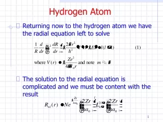
2.1.2 Solution of the radial equation_3 • This shows : • the Schrodinger equation has stationary solutions at energies given by the Bohr formula. • The energy does not depend on l; this accidental degeneracy with different l is a special feature of Coulomb potential. • In contrast, degeneracy with respect to the magnetic quantum number m arises because of the system’s symmetry, i.e. an atom’s properties are independent of its orientation in space, in the absence of external fields. • The solution of the Schrodinger equation gives much more information than just the energies; • From the wave-functions we can calculate other atomic properties in ways that were not possible in the Bohr-Sommerfeld theory.
2.1.2 Solution of the radial equation_4 Examining a few examples of radial wave-functions: Although the energy depends only on n, the shape of the wave-functions depends on both n and l and these two quantum numbers are used to label the radial function. For n=1 there is only the l=0 solution, namely. For n=2 the orbital angular momentum quantum number is l=0 or 1, giving
2.1.2 Solution of the radial equation_6 These show a general a feature of hydrogenic wave-functions, namely that the radial functions for l=0 have a finite value at the origin, i.e. the power series in starts at the zeroth power. Thus electrons with l = 0 (called s-electrons) have a finite probability of being found at the position of the nucleus and this has important consequences in atomic physics.
Exercise • 2.1, 2.2, 2.3, 2.4 2.11