Download
1 / 20
200 likes | 386 Views
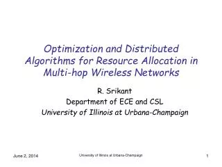
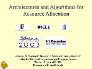
Architectures and Algorithms for Resource Allocation. Mounire El Houmaidi * , Mostafa A. Bassiouni * , and Guifang Li # * School of Electrical Engineering and Computer Science # School of Optics/CREOL University of Central Florida. Outline. Motivation What is a Minimum Dominating Set (MDS)

E N D
Architectures and Algorithms for Resource Allocation Mounire El Houmaidi*, Mostafa A. Bassiouni*, and Guifang Li# *School of Electrical Engineering and Computer Science #School of Optics/CREOL University of Central Florida
Outline • Motivation • What is a Minimum Dominating Set (MDS) • How to find k-MDS • Algorithm • Example • What is Weighted MDS • Applications of k-MDS • Sparse placement of wavelength conversion • k-LOSS(k-BLK) and F-SEARCH • Weighted k-MDS for non-uniform traffic • Limited wavelength conversion • Placement of G-nodes for traffic grooming • Placement of FDLs • Conclusions
24 24 23 23 26 26 7 7 6 6 5 5 11 11 0 0 25 25 22 22 27 27 4 4 8 8 12 12 16 16 21 21 1 1 9 9 13 13 2 2 17 17 20 20 3 3 10 10 14 14 15 15 19 19 18 18 Motivation- Resource placement Optimize overall network performance by using dominating nodes [1-4] (U.S Long Haul Net.) 1. M. El Houmaidi et. al., J. Opt. Net., 2:6, (OSA, 2003) 2. M. El Houmaidi et. al., Proc. MASCOTS, (IEEE/ACM, 2003) 3. M. El Houmaidi et. al., J. Opt. Eng., 43:1, (SPIE, 2004) 4. M. El Houmaidi et. al., Proc. OFC, (IEEE, 2004) Optimize overall network performance by using the dominating nodes (U.S Long Haul topology) • G. Li et. al., JON, 2:6, 2003 • G. Li et. al., JOE, 43:1, 2004 • G. Li et. al., IEEE/ACM MASCOTS, 2003
What is MDS • Given a graph G(V,E), determine a set with minimum number of vertices D V such that every vertex in the graph is either in D or is at distance k or less from at least one member in D. • NP-Complete problem [1,2] . • Heuristic algorithms for sub-optimal solution. • Highly connected nodes dominate the entire topology. 1. Karp, Pl. Press, 1972 2. Lund, et. al., J. ACM, 1994
Definitions • Neighbor (v): is the set of nodes sharing a link with v. • k-Neighbor (v): is the set of nodes that are at most • within k hops away from a node v. • For k equals 0, 0-Neighbor(v) contains the node v only.
Definitions (Cont.) • k-Connect(v): the connectivity index based on nodes within k hops of v is : • k-Master (v): represents the node p, member of k-Neighbor(v), • with the highest k-Connect value over all nodes m that are at • most k hops away from node v (i.e., all nodes mk-Neighbor(v))
k-WMDS Algorithm • Initialize the dominating set k-WMDS to . • For all nodes v in G, Compute k-Connect (v). • Each node v sends CON(v) with computed k-Connect(v) to • all nodes in k-Neighbor (v). • Each node v finds its k-Master(v), denoted node m, based on • the values received in CON messages. • Each node v sends VOTE(v) message to m=k-Master(v). • The VOTE message informs node m that it is a master node . • Each node that receives VOTE(v) adds itself to k-WMDS.
24 23 26 7 6 5 11 0 25 22 27 4 8 12 16 21 1 9 13 2 17 20 3 10 14 15 19 18 U.S Long Haul network 1-MDS (USLH) = {1, 3, 4, 5, 8, 10, 12, 15,17, 20, 22, 25, 27} 2-MDS (USLH) = {4, 8, 12, 17, 25} (double circled in graph) 3-MDS (USLH) = {8, 12, 17} 4-MDS (USLH) = {12}
Comparing k-MDS vs. k-LOSS (k-BLK) load=60,k-MDSk-BLK k=3 17% (32%) 20% (20%) k=2 13% (48%) 19% (24%) k=17% (72%) 10% (60%) We can achieve almost 50% improvement with only 5 nodes
NSFNET: nationwide backbone network 15 12 11 9 3 14 8 1 7 4 6 13 0 10 2 5 Weighted MDS (k-WMDS) 0-Connect (v) = Cardinality (Neighbor (v)) * Weight(v) 1-WMDS (NSF) = {1, 4, 5, 6, 9, 11, 14} 2-WMDS (NSF) = {1, 4, 9, 14} 3-WMDS (NSF) = {14}
k-LOSS (k-BLK) vs. k-WMDS Under a load of 70, we simulated non-uniform traffic pattern between node pairs: Node Weight 0 6 1 12 2 7 3 12 4 5 5 8 6 1 7 11 8 7 9 2 10 7 11 15 12 3 13 15 14 9 15 2
Placement of Limited OWC LIMITED has better performance than F-SEARCH forFlexible node-sharing and Static mapping optical switch designs.
G-nodes placement: T-Grooming We can achieve with 2-WMDS members as G-nodes (r=16) the same throughput as if all nodes in the network had the grooming capability (r is the grooming ratio) G-nodes placement for traffic Grooming We can achieve with 2-WMDS members as G-nodes (r=16) the same throughput as if all nodes had the grooming capability (r is the grooming ratio)
OBS switch design with FDLs/OWCs MAIN CONTROL Input Link 1 DMX 1 Converter Bank A 1 B 1 C 1 1 MUX Output Link 1 OWC W 1 C 2 C 1 A 1 . . . W W OWC O X C Input Link 2 DMX Converter Bank i MUX Output Link 2 1 A 2 B 2 C 2 OWC B 1 A 2 B 2 F.W . . . W OWC F.W + 1 F.W + 1 DMX: De-multiplexor MUX: Multiplexor OWC: any-to- Converter FDL: Fiber Delay Line F.W + 2 F.W + 2 FDL Bank 2 FDL 1 FDL
λ1 . . . λW λ1 . . . λW 22 21 20 2(max_d) OWC OWC … … OWC OWC Fiber Delay Line design Variable delay: [0…MAXD], where MAXD = (20 + 21 +… +2(max_d)) x b
Benefits of FDLs and OWCs FDLs vs. OWCs with JET signaling and W=16
Efficient FDLs/OWCs placement • In a fully connected network (all nodes are connected), OWC has no effect on the blocking performance but FDLs do. • FDLs and OWCs capabilities must be used judiciously and placed in nodes that maximize the performance. • k-LOSS heuristic [JIM99, MSS02]: Via simulation, Place OWC in nodes experiencing the highest blocking rates.
Conclusion • k-MDS provides an efficient sparse OWC placement. • k-WMDS models non-uniform traffic patterns. • k-MDS allows efficient placement of limited OWC. • It applies to G-nodes selection for traffic grooming. • k-WMDS efficiently place FDLs.
Discussion and Questions