Download
1 / 23
230 likes | 361 Views
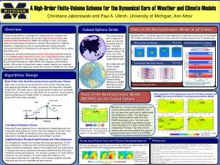
A Look at High-Order Finite-Volume Schemes for Simulating Atmospheric Flows. Paul Ullrich University of Michigan. Next Generation Climate Models. High-order accurate Move away from latitude-longitude grids Utilize modern hardware (GPUs, Petascale computing) Adaptive mesh refinement?.

E N D
A Look at High-Order Finite-Volume Schemes for Simulating Atmospheric Flows Paul UllrichUniversity of Michigan
Next Generation Climate Models • High-order accurate • Move away from latitude-longitude grids • Utilize modern hardware (GPUs, Petascale computing) • Adaptive mesh refinement?
The Cubed Sphere Grid • The cubed sphere grid is obtained by placing a cube inside the sphere and “inflating” it to occupy the total volume of the sphere. • Pros: • Removes polar singularities • Grid faces are individually regular • Cons • Some difficulty handling edges • Multiple coordinate systems • Many atmospheric models now utilize this grid.
Why Finite Volumes? • Finite volume methods have several advantages over finite difference and spectral methods: • They can be used to conserve invariant quantities, such as mass, energy, potential vorticity or potential enstrophy. • Finite volume methods can be easily made to satisfy monotonicity and positivity constraints (i.e. to avoid negative tracer densities). • Lots of research has been done on finite volume methods in aerospace and other CFD fields.
Unstaggered vs. Staggered Grids • Many atmospheric models make use of staggered grids (ie. Arakawa B,C,D-grids), where velocity components and mass-variables are located at different grid points. • Staggered grids have certain advantages, such as better treatment of high-wavenumber wave modes. • However, staggered grids have stricter timestep constraints. • Unstaggered grids allow us to easily perform horizontal-vertical dimension splitting. • Staggered grids also suffer from unphysical wave reflection at abrupt grid resolution discontinuities (on adaptive grids)…
Finite Volume Formulation • The high-order upwind finite volume model consists of several components, a few of which will be covered here: The sub-grid-scale reconstruction The Riemann solver The implicit-explicit dimension-split integrator 1 2 3
Sub-Grid Scale Reconstruction 1 Our sub-grid scale reconstruction can use only information on the cell-averaged values within each element. Cell 1 Cell 2 Cell 3 Cell 4
Sub-Grid Scale Reconstruction 1 The least accurate and least computation-intensive method for building a sub-grid scale reconstruction assumes that all points within a source grid element share the same value. Cell 1 Cell 2 Cell 3 Cell 4 Piecewise ConstantMethod (PCoM)
Sub-Grid Scale Reconstruction 1 Increasing the accuracy of the method with respect to the reconstruction simply requires using increasingly high order polynomials for the sub-grid scale reconstruction. Cell 1 Cell 2 Cell 3 Cell 4 A cubic reconstruction will lead to a 4th order accurate scheme, if paired with a sufficiently accurate timestep scheme. Piecewise CubicMethod (PCM)
The Riemann Solver 2 Since the reconstruction is inherently discontinuous at cell interfaces, we must solve a Riemann problem to obtain the flux of all conserved variables. UL UR Cell 1 Cell 2
The Riemann Solver 2 A crude choice of Riemann solver can result in excess diffusion, which can severely contaminate the solution. Rusanov Riemann solver AUSM+-up Riemann solver
Results: Shallow Water Model Williamson et al. (1992) Test Case 2 - Steady State Geostrophic Flow (=45) Fluid Depth (h)
Results: Shallow Water Model Williamson et al. (1992) Test Case 5 - Flow over Topography Total Fluid Depth (H)
Vertical Discretization 3 Vertically propagating sound waves are a major issue for nonhydrostatic models. This suggests special treatment is required of the vertical coordinate. • Idea: Since we are using an unstaggered grid, its easy to split the horizontal and vertical integration and treat the vertical integration implicitly, even in the presence of topography. • Since vertical columns are disjoint, each column only requires a single implicit solve; total matrix size = 5 x <# of vertical levels>. • In order to achieve high-order accuracy we use Implicit-Explicit Runge-Kutta-Rosenbrock (IMEX-RKR) schemes. • The resulting method is valid on all scales, uses the horizontal timestep constraint, is high-order accurate and is only modestly slower than a hydrostatic model.
Vertical Discretization 3 Care must be taken to choose a high-order-accurate timestepping scheme. Poor choices can lead to severely degraded model results. 1,2,3. Explicit steps 4. Implicit step 1,3,5. Explicit steps 2,4. Implicit steps
Results: 3D Nonhydrostatic Model Jablonowski (2011) Baroclinic Instability in a Channel Temperature at 500m
Summary • Next generation atmospheric models will likely rely on high-order numerical methods to achieve accuracy at a reduced computational cost. • We have successfully demonstrated a high-order finite volume method for the shallow-water equations on the sphere and for nonhydrostatic 2D and 3D modeling. • Implicit-explicit Runge-Kutta-Rosenbrock (IMEX-RKR) methods are very good candidates for time integrators, and can likely be adapted to any unstaggered grid model (high-order FV, DG, SV).
The Riemann Solver 2 The Riemann solver introduces a natural source of damping, which can act to suppress oscillations in the divergence. Example: Third-order reconstruction (parabolic sub-grid-scale) applied to the linear shallow-water equations plus Riemann solver. Advective Term (proportional to dm/dx) Diffusive Term (proportional to c dh4/dx4)
Next Generation Climate Models ShallowWater Hydro-static Nonhydro-static Advection Finite Volume High-order upwind High-order symmetric Compact Stencil Discontinuous Galerkin Spectral element / CG Spectral volume Semi-Lagrangian