16.451 Lecture 7: Understanding the cross-section results 25/9/2003

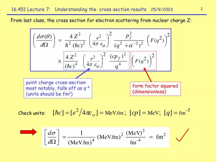
1. point charge cross-section: most notably, falls off as q-4 (units should be fm2) form factor squared (dimensionless) Check units: 16.451 Lecture 7: Understanding the cross-section results 25/9/2003 1 From last class, the cross section for electron scattering from nuclear charge Z:

2. point charge constants: For the kinematic factors, we need our results from lecture 5 for the momenta, being of course very careful with the units: What does this function look like? 2 First calculate the point charge cross section for Z = 1:

3. pf pi (ħq)2 Kinematic relations become: 208Pb, pi= 248 MeV/c Point charge cross section, continued... 3 First, let’s consider a heavy nuclear target, so that pf pi and work out Z2d/d)o Choose the example of 248 MeV/c electrons scattering from 208Pb as in Krane, fig. 3.2

4. Point charge calculation for 248 MeV/c electrons scattering from 208Pb, Z = 82... 4 NB, the graph blows up at  = 0. In this limit, the practical cutoff is given by -2, a scale set by the size of the atom.... Log scale! The point charge cross section drops like a stone!!!

5. (F(q2))2 at 10° = 10/982 = 0.01 !!! How are we doing? Compare to data from Krane: 5  = 10°, d/d = 105 b/sr = 10 fm2/sr ... Point charge calculation: d(10°)/d = 982 fm2/sr Also, the graphs are not smooth like 1/q4 -- evidence that the target has finite size!

6. Recall our basic result from lecture 6: Where F(q2) is the Fourier transform of the target charge density: Measuring d/d and dividing by the point charge result yields a value for F(q2) Summary so far: 6 We can predict the cross-section exactly for a pointlike target with nonrelativistic quantum mechanics. (This approach is correct for a target particle that has charge but no magnetic moment, i.e. intrinsic angular momentum of zero. We can’t use this for the proton without adding some refinements, so along the way we are stopping to look at the charge distributions of nuclei. Nuclei with (Z, N) both even, such as 208Pb, have angular momentum zero, so our theory is perfect for this case!)

7. inverse Fourier transform: How to find the charge distribution? 7 form factor: In principle, one could measure the form factor, and numerically integrate to invert the Fourier transform and find (r). However, this doesn’t work in practice, because the integral has to be done over a complete range of q from 0 to ∞, and no experiment can ever span an infinite range of momentum transfer! (It is bad enough trying to acquire data at large momentum transfer because the basic cross-section drops like q-4  the rate of scattered particles into a detector gets too small – see slide 14, lecture 4) What to do? ...

8. Discontinuities are evidence of diffraction-like behavior, characteristic of a Fourier transform, but the edges are fuzzy! A practical solution: 8 Experimental data are fitted to a functional form for F(q2); parameters extracted from the fit are used to invert the transform and deduce (r).... Example: elastic electron scattering from gold (A=197, Z = 79). Best fit to data is given by solid curves. (Ref: R. Hofstadter, Electron Scattering & Nuclear Structure, 1963)

9. Density: Zeroes never quite get to zero on a log scale! Illustration of “Diffraction” behavior in F(q2): Uniform sphere 9 In contrast, the minima are not as sharp for nuclei...

10. Nuclear charge distributions from experiment: 10 diffuse surface excludes sharp diffraction minima Approx. constant central density

11. Electric charge distribution: Proton Form factor data: Contrast to the proton (recall lecture 4): 11