Download
1 / 46
520 likes | 792 Views
Analysis of Survival Data. Time to Event outcomes Censoring Survival Function Point estimation Kaplan-Meier. Introduction to survival analysis. What makes it different? Three main variable types Continuous Categorical Time-to-event Examples of each.

E N D
Analysis of Survival Data Time to Event outcomes Censoring Survival Function Point estimation Kaplan-Meier
Introduction to survival analysis • What makes it different? • Three main variable types • Continuous • Categorical • Time-to-event • Examples of each
Example: Death Times of Psychiatric Patients (K&M 1.15) • Dataset reported on by Woolson (1981) • 26 inpatient psychiatric patients admitted to U of Iowa between 1935-1948. • Part of larger study • Variables included: • Age at first admission to hospital • Gender • Time from first admission to death (years)
Data summary . tab gender gender | Freq. Percent Cum. ------------+----------------------------------- 0 | 11 42.31 42.31 1 | 15 57.69 100.00 ------------+----------------------------------- Total | 26 100.00 gender age deathtime death 1 51 1 1 1 58 1 1 1 55 2 1 1 28 22 1 0 21 30 0 0 19 28 1 1 25 32 1 1 48 11 1 1 47 14 1 1 25 36 0 1 31 31 0 0 24 33 0 0 25 33 0 1 30 37 0 1 33 35 0 0 36 25 1 0 30 31 0 0 41 22 1 1 43 26 1 1 45 24 1 1 35 35 0 0 29 34 0 0 35 30 0 0 32 35 1 1 36 40 1 0 32 39 0 . sum age Variable | Obs Mean Std. Dev. Min Max -------------+-------------------------------------------------------- age | 26 35.15385 10.47928 19 58
Death time? . sum deathtime Variable | Obs Mean Std. Dev. Min Max -------------+-------------------------------------------------------- deathtime | 26 26.42308 11.55915 1 40
Does that make sense? . tab death death | Freq. Percent Cum. ------------+----------------------------------- 0 | 12 46.15 46.15 1 | 14 53.85 100.00 ------------+----------------------------------- Total | 26 100.00 • Only 14 patients died • The rest were still alive at the end of the study • Does it make sense to estimate mean? Median? • How can we interpret the histogram? • What if all had died? • What if none had died?
CENSORING • Different types • Right • Left • Interval • Each leads to a different likelihood function • Most common is right censored
Right censored data • “Type I censoring” • Event is observed if it occurs before some prespecified time • Mouse study • Clock starts: at first day of treatment • Clock ends: at death • Always be thinking about ‘the clock’
Introduce “administrative” censoring Time 0 STUDY END
Introduce “administrative” censoring Time 0 STUDY END
More realistic: clinical trial “Generalized Type I censoring” Time 0 STUDY END
More realistic: clinical trial “Generalized Type I censoring” Time 0 STUDY END
Additional issues • Patient drop-out • Loss to follow-up
Drop-out or LTFU Time 0 STUDY END
How do we ‘treat” the data? Shift everything so each patient time represents time on study Time of enrollment
Another type of censoring:Competing Risks • Patient can have either event of interest or another event prior to it • Event types ‘compete’ with one another • Example of competers: • Death from lung cancer • Death from heart disease • Common issue not commonly addressed, but gaining more recognition
Left Censoring • The event has occurred prior to the start of the study • OR the true survival time is less than the person’s observed survival time • We know the event occurred, but unsure when prior to observation • In this kind of study, exact time would be known if it occurred after the study started • Example: • Survey question: when did you first smoke? • Alzheimers disease: onset generally hard to determine • HPV: infection time
Interval censoring • Due to discrete observation times, actual times not observed • Example: progression-free survival • Progression of cancer defined by change in tumor size • Measure in 3-6 month intervals • If increase occurs, it is known to be within interval, but not exactly when. • Times are biased to longer values • Challenging issue when intervals are long
Key components • Event: must have clear definition of what constitutes the ‘event’ • Death • Disease • Recurrence • Response • Need to know when the clock starts • Age at event? • Time from study initiation? • Time from randomization? • time since response? • Can event occur more than once?
Time to event outcomes • Modeled using “survival analysis” • Define T = time to event • T is a random variable • Realizations of T are denoted t • T 0 • Key characterizing functions: • Survival function • Hazard rate (or function)
Survival Function • S(t) = The probability of an individual surviving to time t • Basic properties • Monotonic non-increasing • S(0)=1 • S(∞)=0* * debatable: cure-rate distributions allow plateau at some other value
Applied example Van Spall, H. G. C., A. Chong, et al. (2007). "Inpatient smoking-cessation counseling and all-cause mortality in patients with acute myocardial infarction." American Heart Journal 154(2): 213-220. Background Smoking cessation is associated with improved health outcomes, but the prevalence, predictors, and mortality benefit of inpatient smoking-cessation counseling after acute myocardial infarction (AMI) have not been described in detail. Methods The study was a retrospective, cohort analysis of a population-based clinical AMI database involving 9041 inpatients discharged from 83 hospital corporations in Ontario, Canada. The prevalence and predictors of inpatient smoking-cessation counseling were determined. Results….. Conclusions Post-MI inpatient smoking-cessation counseling is an underused intervention, but is independently associated with a significant mortality benefit. Given the minimal cost and potential benefit of inpatient counseling, we recommend that it receive greater emphasis as a routine part of post-MI management.
Applied example Adjusted 1-year survival curves of counseled smokers, noncounseled smokers, and never-smokers admitted with AMI (N = 3511). Survival curves have been adjusted for age, income quintile, Killip class, systolic blood pressure, heart rate, creatinine level, cardiac arrest, ST-segment deviation or elevated cardiac biomarkers, history of CHF; specialty of admitting physician; size of hospital of admission; hospital clustering; inhospital administration of aspirin and β-blockers; reperfusion during index hospitalization; and discharge medications.
Hazard Function • A little harder to conceptualize • Instantaneous failure rate or conditional failure rate • Interpretation: approximate probability that a person at time t experiences the event in the next instant. • Only constraint: h(t)0 • For continuous time,
Hazard Function • Useful for conceptualizing how chance of event changes over time • That is, consider hazard ‘relative’ over time • Examples: • Treatment related mortality • Early on, high risk of death • Later on, risk of death decreases • Aging • Early on, low risk of death • Later on, higher risk of death
Shapes of hazard functions • Increasing • Natural aging and wear • Decreasing • Early failures due to device or transplant failures • Bathtub • Populations followed from birth • Hump-shaped • Initial risk of event, followed by decreasing chance of event
Median • Very/most common way to express the ‘center’ of the distribution • Rarely see another quantile expressed • Find t such that • Complication: in some applications, median is not reached empirically • Reported median based on model seems like an extrapolation • Often just state ‘median not reached’ and give alternative point estimate.
X-year survival rate • Many applications have ‘landmark’ times that historically used to quantify survival • Examples: • Breast cancer: 5 year relapse-free survival • Pancreatic cancer: 6 month survival • Acute myeloid leukemia (AML): 12 month relapse-free survival • Solve for S(t) given t
Competing Risks • Used to be somewhat ignored. • Not so much anymore • Idea: • Each subject can fail due to one of K causes (K>1) • Occurrence of one event precludes us from observing the other event. • Usually, quantity of interest is the cause-specific hazard • Overall hazard equals sum of each hazard:
Example • Myeloablative Allogeneic Bone Marrow Transplant Using T Cell Depleted Allografts Followed by Post-Transplant GM-CSF in High Risk Myelodysplastic Syndromes • Interest is in RELAPSE • Need to account for treatment related mortality (TRM)? • Should we censor TRM? • No. that would make things look more optimistic • Should we exclude them? • No. That would also bias the results • Solution: • Treat it as a competing risk • Estimate the incidence of both
Estimating the Survival Function • Most common approach abandons parametric assumptions • Why? • Not one ‘catch-all’ distribution • No central limit theorem for large samples
Censoring • Assumption: • Potential censoring time is unrelated to the potential event time • Reasonable? • Estimation approaches are biased when this is violated • Violation examples • Sick patients tend to miss clinical visits more often • High school drop-out. Kids who move may be more likely to drop-out.
Terminology • D distinct event times • t1 < t2 < t3 < …. < tD • ties allowed • at time ti, there are di deaths • Yi is the number of individuals at risk at ti • Yi is all the people who have event times ti • di/Yi is an estimate of the conditional probability of an event at ti, given survival to ti
Kaplan-Meier estimation • AKA ‘product-limit’ estimator • Step-function • Size of steps depends on • Number of events at t • Pattern of censoring before t
Kaplan-Meier estimation • Greenwood’s formula • Most common variance estimator • Point-wise
Example: • Kim paper • Event = time to relapse • Data: • 10, 20+, 35, 40+, 50+, 55, 70+, 71+, 80, 90+
Interpreting S(t) • General philosophy: bad to extrapolate • In survival: bad to put a lot of stock in estimates at late time points
Fernandes et al: A Prospective Follow Up of Alcohol Septal Ablation For Symptomatic Hypertrophic Obstructive Cardiomyopathy The Ten-Year Baylor and MUSC Experience (1996-2007)”
R for KM library(survival) library(help=survival) t <- c(10,20,35,40,50,55,70,71,80,90) d <- c(1,0,1,0,0,1,0,0,1,0) cbind(t,d) st <- Surv(t,d) st help(survfit) fit.km <- survfit(st) fit.km summary(fit.km) attributes(fit.km) plot(fit.km, conf.int=F, xlab="time to relapse (months)", ylab="Survival Function“, lwd=2)