Download

1 / 44
630 likes | 904 Views
Survival Analysis. Survival Analysis. Statistical methods for analyzing longitudinal data on the occurrence of events.

E N D
Survival Analysis • Statistical methods for analyzing longitudinal data on the occurrence of events. • Events may include death, injury, onset of illness, recovery from illness (binary or dichotomous variables) or transition above or below the clinical threshold of a meaningful continuous variable (e.g. CD4 counts). • Accommodates data from randomized clinical trial or cohort study design.
Intervention Control Randomized Clinical Trial (RCT) Disease Random assignment Disease-free Target population Disease-free, at-risk cohort Disease Disease-free TIME
Treatment Control Randomized Clinical Trial (RCT) Cured Random assignment Not cured Target population Patient population Cured Not cured TIME
Treatment Control Randomized Clinical Trial (RCT) Dead Random assignment Alive Target population Patient population Dead Alive TIME
Survival analysis • Primary focus is ‘time-to-event’ or “survival” time • e.g time until death, time until recurrence, time until remission, time until CD4 count declines or drops below a certain level etc. • Events may include all kinds of “positive” or “negative’”eventse.g. Time until tumor shrinks 20%, time until death, time until an alcoholic relapses and begins drinking again, etc. • Can use single and combined endpointse.g time until death or time until CD4 count declines are single endpoints while time until either CD4 count declines or death occurs is a combined endpoint. • Problem: the event of interest may never be observed!
Censoring • Most survival analyses must deal with a key problem called censoring. • Censoring occurs when the event of interest is not observed for whatever reason so we do not know the exact “survival” time. There are generally three reasons why censoring occurs: • a person does not experience the event before the study ends. • a person is lost to follow-up during the study period. • a person “withdraws” from the study for whatever reason.
Patients Patients Status Status 1 1 start of RRT recovery of renal function recovery of renal function censored censored start of RRT start of RRT 2 2 censored censored 3 3 start of RRT start of RRT death death event event 4 4 start of RRT start of RRT censored death due to competing cause death death 5 5 event event start of RRT start of RRT 6 6 event event death death start of RRT start of RRT 7 7 censored censored start of RRT start of RRT loss to follow loss to follow - - up up 8 8 event event start of RRT start of RRT death death 31 31 - - 12 12 - - 2005 2005 01 01 - - 01 01 - - 1996 1996 31 31 - - 12 12 - - 2000 2000 The incidence rate of death for renal replacement therapy (RRT) patients Example – Survival time on RRT: events & censored observations ____________________________________________________________ Incident RRT patients in the ERA-EDTA Registry were included in an analysis of patient survival on RRT. Like in most survival studies patients were recruited over a period of time (1996-2000 - the inclusion period) and they were observed up to a specific date (31 December 2005 - the end of the follow-up period). During this period the event of interest was ‘death while on RRT’, whereas censoring took place at recovery of renal function, loss to follow-up and at 31 December 2005. End Start Survival times of eight patients at risk of death on RRT. The inclusion period was 1996-2000, whereas follow-up was ended on 31 December 2005.
Assumptions related to censoring • At any time patients who are censored have the same survival prospects as those who continue to be followed. • This sometimes is problematic: e.g. in the calculation of survival on dialysis censoring at the time of transplantation is needed because these patients are no longer at risk of death on dialysis – however dialysis patients on the transplant waiting list do not have the same prospects as dialysis patients who are not on the waiting list • Survival probabilities are assumed to be the same for subjects recruited early and late in the study. • May test this by splitting a cohort of patients in those who were recruited early and those recruited late and see if their survival curves are different.
Kaplan Meier method • Used to estimate survival probabilities and to compare survival of different groups. Example 2 - Survival probability in RRT patients due to diabetes mellitus and other causes In a sample of 50 RRT patients taken from a study on diabetes mellitus survival time started running at the moment a patient was included in the study, in this case at the start of RRT. Patients were followed until death or censoring. The survival probability was calculated using the Kaplan Meier method. Subsequently, the survival of patients with ESRD due to diabetes mellitus was compared to the survival of those with ESRD due to other causes. • Observed survival times are first sorted in ascending order, starting with the patient with the shortest survival time and presented in a table.
Kaplan Meier method • At the start of the study all 50 patients were alive - proportion surviving and cumulative survival were 1.00 • When the first patient died on day 34 after the start of RRT, the proportion surviving was 49/50 = 0.9800 = 98%. To calculate the cumulative survival this proportion surviving was multiplied by the 1.0 cumulative survival from the previous step resulting in a cumulative survival dropping to 0.9800. • When the second patient died at day 35, the proportion surviving was 48/49 = 0.9796. To obtain the cumulative survival at day 35, again, this proportion was multiplied by the 0.9800 cumulative survival from the previous step which resulted in a cumulative survival dropping that day to 0.9600. • On day 57, however, a patient was withdrawn alive from the study (censored). The proportion surviving that day was 47/47 = 1.00, as this patient did not die but was withdrawn alive from the study. As a result the cumulative survival did not drop that day but remained unchanged at 0.9400.
Kaplan Meier method • Cumulative survival is a probability of surviving the next period multiplied by the probability of having survived the previous period • All subjects at risk - also those not experiencing the event during the observation period - can contribute survival time to the denominator of the incidence rate • By censoring one is able to reduce the • number of persons alive without • affecting the cumulative survival
Kaplan Meier method • The median survival is that point in time, from the time of inclusion, when the cumulative survival drops below 50%, in this case it is 1708 days • Is not related to the number of deaths or the number of subjects that is still at risk • Why mean survival is used less frequently: • Survival data mostly highly skewed. • In case of censoring one does not know if and when the person will experience the event – this complicates the calculation of the mean. • In order to calculate a mean survival one would need to wait until all persons experienced the event.
Log-rank Test P = 0.04 • Most popular method of comparing the survival of groups. • Takes the whole follow-up period into account. • Addresses the hypothesis that there are no differences between the populations being studied in the probability of an event at any time point.
Example: Remission time of acute leukemia • Purpose: evaluate drug’s ability to maintain remissions • Patients randomly assigned • Study terminated after 1 year • Different follow up times due to sequential enrollment • 6-MP • 6,6,6,7,10,22,23,6+,9+,10+,11+,17+,19+,20+,25+,32+,32+,34+,35+ • Placebo • 1,1,2,2,3,4,4,5,5,8,8,8,8,11,11,12,12,15,17,22,23
Example: Remission time of acute leukemia 6-MP(Group = 1) 6,6,6,6+,7,9+,10,10+,11+,17+,19+,20+,22,23,25+,32+,32+,34+,35+ Placebo(Group = 2) 1,1,2,2,3,4,4,5,5,8,8,8,8,11,11,12,12,15,17,22,23 In JMP (1 is used to denote censored times, 0 for non-censored) E.g. for Group 1 – first 8 observations6, 6, 6, 6+, 7, 9+, 10, 10+
Example: Remission time of acute leukemia Group 1 – 6-MP Group 2 - Placebo We can clearly see that the time until remission (“survival”) time is larger for the treatment (6-MP) group than control. The log-rank and Wilcoxon tests for comparing the “survival” experience of both groups suggest a statistically significant difference exist (p < .0001).
Retrospective cohort study:From December 2003 BMJ: Aspirin, ibuprofen, and mortality after myocardial infarction: retrospective cohort study
What the Kaplan Meier method and the log-rank test can and cannot do… • Together the Kaplan Meier method and the logrank test provide an opportunity to: • Estimate survival probabilities and • Compare survival between groups • However • One cannot adjust for confounding variables – i.e. no mutlivariate analysis • They do not provide an estimate of the effect size and the relating confidence interval • → In those cases one needs a regression technique like the • Cox proportional hazards model (Cox PH Model)
Cox Proportional Hazard Model • Before we can talk about the Cox PH model we need to consider some characteristics and terminology associated with survival time distributions. • Here survival times might be time until death, but these times can also represent other outcomes such as time until remission, time until relapse, etc.
Introduction to survival distributions • Tithe event time for an individual, is a random variable having a probability distribution. • Different models for survival data are distinguished by different choices for thedistribution of Ti.
Describing Survival Distributions The idea is this: Assume that times-to-event for individuals in your dataset follow a continuous probability distribution (typically a skewed right distribution, generally not normal!). For all possible times Ti after baseline, there is a certain probability that an individual will have an event at exactly time Ti. For example, human beings have a certain probability of dying at ages 3, 25, 80, and 140: P(T=3), P(T=25), P(T=80), and P(T=140). These probabilities are obviously vastly different.
People have a high chance of dying in their 70’s and 80’s; BUT they have a smaller chance of dying in their 90’s and 100’s, because few people make it long enough to die at these ages. Probability density function: f(t) In the case of human longevity, Ti is unlikely to follow a normal distribution, because the probability of death is not highest in the middle ages, but at the beginning and end of life. Hypothetical data:
Probability density function: f(t) Show’s how failure times are distributed. If we had no censoring a histogram of the survival times of say ESRD patients would give us an impression of what the probability density function, f(t), looks like. The smoothed curve added to the histogram is a visualization of f(t) based upon a sample of patients with ESRD.
F(t) is the CDF of f(t), and is “more interesting” than f(t). Survival function: 1 - F(t) The goal of survival analysis is to estimate and compare survival experiences of different groups. Survival experience is described by the cumulative survival function: Example: If t = 100years, S(100) = S(t=100) which is the probability of surviving beyond 100 years.
Cumulative Survival Same hypothetical data, plotted as cumulative distribution rather than density: Recall f(t)
Cumulative survival, S(t) = P(T >t) S(20) = P(T>20) S(80) = P(T>80)
AGES Hazard Function h(t): a new concept Hazard rate is an instantaneous incidence rate. Think of it like the rate of change of your chance of dying, like a speedometer on a car racing towards death.
Hazard function h(t) In words: the probability that if you survive to t, you will succumb to the event in the next instant.
Hazard h(t) vs. Density f(t) This is subtle, but the idea is: • When you are born, you have a certain probability of dying at any age; that’s the probability density. • Example: a woman born today has, say, a 1% chance of dying at 80 years. • However, as you survive for awhile, your probabilities keep changing (think: conditional probability) • Example, a woman who is 79 today has, say, a 5% chance of dying at 80 years.
A possible set of probability density, failure, survival, and hazard functions. f(t)=density function F(t)=cumulative failure = P(T < t) S(t)=cumulative survival h(t)=hazard function
Cox Proportional Hazards Model • Model for the hazard function as a function of covariates/predictors/independent variables. • The interpretation of the estimated coefficients in the model is similar to the coefficients in a logistic regression model. • Logistic Regression Odds Ratios (OR) • Cox PH Model Hazard Ratio (HR) In order to understand the distinction between OR’s and HR’s we need to discuss the difference between incidence rates and proportions.
Incidence Rate vs. Proportion • Incidence (hazard) rate - number of new cases of disease per population at-risk per unit time (or mortality rate, if outcome is death). • Cumulative incidence - proportion of new cases that develop in a given time period • Hazard or rate ratio (HR) is the ratio of incidence rates. • Odds or risk ratio (OR or RR) is the ratio of proportions.
Cox Proportional Hazards Model The Cox PH Model for individuals with k covariate values says the hazard function for these individuals is given by: where is the baseline hazard function which is assumed to be the same for all individuals. The covariates then multiple the baseline hazard to give a covariate specific hazard function.
Hazard Ratio (HR) Consider the population i which consists of all individuals with k covariate values and population j which consists of all individual with k covariate values then the hazard ratio for comparing population i to population j individuals is given by:
Hazard Ratio (HR) – for dichotomous covariates Example 1: Suppose we are modeling the hazard function for developing lung cancer using smoking status and age as covariates. Find the HR for 60-year old smokers (+1, ) vs. non-smokers (-1 , ). Thus the HR associated with smoking for 60-year old individuals is . Notice the similarity to the interpretation of coefficients in a logistic regression model.Note: The particular age is irrelevant as long as it is the same for both populations being compared.
Hazard Ratio (HR) – for continuous covariates Example 2: Suppose we are modeling the hazard function for developing lung cancer using smoking status and age as covariates. Find the HR for 70-year old smokers (+1, ) vs. 60-year old smokers (). Thus the HR associated with a 10-year increase in age starting at age 60 is . Notice the similarity to the interpretation of coefficients for continuous variables in a logistic regression model. Note: This would be the same if we compared any two ages that are 10-years apart. Also smoking status irrelevant if it is the same for both populations we are considering.
Example: Remission time for acute leukemia Here we have two dichotomous covariates in a Cox PH model for remission time. The hazard ratio (HR) for females is then given by .752, so females have less risk of remission than males. The hazard ratio (HR) for males is the reciprocal 1/.752 = 1.33, so males have 1.33 times the risk of remission. These are only point estimates however, thus we also need to consider CI’s.
Example: Remission time for acute leukemia Here we have two dichotomous covariates in a Cox PH model for remission time. The hazard ratio (HR) for receiving the active treatment (6-MP) is given by and the hazard ratio (HR) for those receiving placebo is therefore 1/.2005 = 4.988, thus those receiving placebo have 5 times the risk for remission. Again we should examine CI’s for these HR’s.
Example: Remission time for acute leukemia Here we have one continuous covariate in the Cox PH model for remission time. log of the white blood cell count The estimate coefficient for the log base 2 of the white blood cell count is 1.59. A unit increase in corresponds to doubling the WBC, so if we compare two populations patients, one with double the WBC of the other the estimated HR is given by So the population with double the WBC has 4.92 times the risk of remission. Next we consider a Cox PH model using treatment, sex, and as covariates.
Example: Remission time for acute leukemia Next we consider a Cox PH model using treatment, sex, and as covariates. We can see that both Treatment and log2WBC are statistically significant, while Sex of the patient is not. JMP can be used to calculate the Risk Ratios or Hazard Ratios (HR). The estimated HR associated with not receiving the 6-MP therapy is 4.02 with a CI (1.698, 10.307) and the estimated HR associated with doubling the WBC is 4.92 with a CI (2.65, 9.73).
Example: Remission time for acute leukemia Next we consider a Cox PH model using treatment, sex, and as covariates. We can see that both Treatment and log2(WBC) are statistically significant, while Sex of the patient is not. JMP can be used to calculate the Risk Ratios or Hazard Ratios (HR). The estimated HR for males vs. females is 1.30, however the CI includes 1, so we cannot say there is increased risk of recurrence for males. This is further supported by the p-value = .5596.
Summary of Survival Analysis Survival analysis involves making inferences about the time until event occurs. Due to the prospective nature of these studies there are frequently censored time observations. The Kaplan-Meier Method allows us to describe both visually and numerically the survival experience of subjects in our study. The log-rank test allows us to compare the survival experience of subjects across treatment groups. The Cox Proportional Hazards Model allows us to examine the relationship between the survival experience of subjects and covariates that might be related to their survival; or to look at group/treatment differences adjusted for other covariates.