Download
1 / 23
230 likes | 316 Views
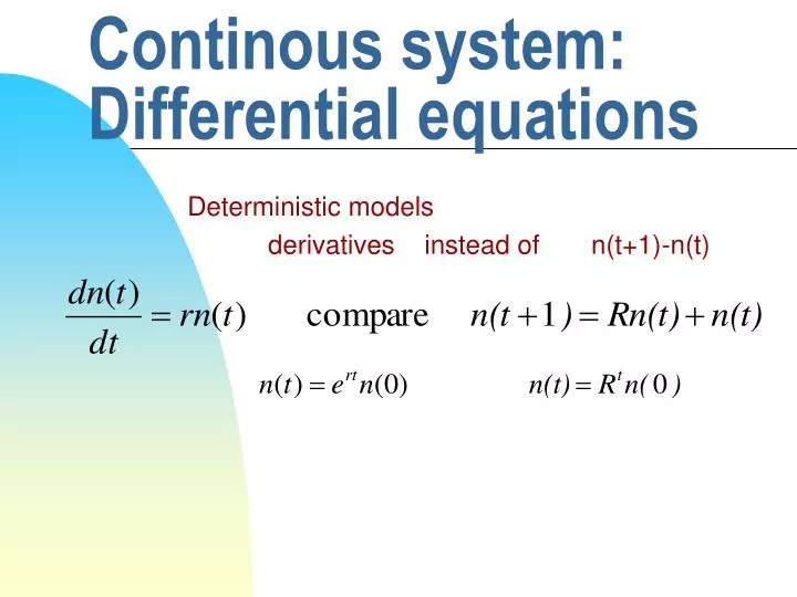
Continous system: Differential equations. Deterministic models derivatives instead of n(t+1)-n(t). Determine the equation. Decide what have an effect on the system Determine whether the parameters are positive or negative, i. e. give growth or reduction

E N D
Continous system: Differential equations Deterministic models derivatives instead of n(t+1)-n(t)
Determine the equation • Decide what have an effect on the system • Determine whether the parameters are positive or negative, i. e. give growth or reduction • Determine whether the parameter is linear or nonlinear in relation to your entity (often population density or amount of a compound) rx Population x growth -dx bx Population x deaths birth immigration i
Determine the equation rx Population x • What act on the system, entity: sign, constant or linear/nonlinear relation: rx is positive, linear • What act on the system, entity: sign, constant or linear/nonlinear relation: bx, positive, linear dx, negative, lineari, positive, constant tillväxt -dx bx Population x deaths birth immigration i
Differential equations, part 2 • Geometrical analysis • Nonlinear Differential Equations
What is differential equations? • Derivatives in an equation, i e both y and y’ in the very same equation • Example: Both concentration and change of concentration • To solve this one how to maken some kind of integration, that is make y’ to y. • Note: most of the differential equations is not possible to solve analytically, one is referred to numerical solutions
Geometric analysis: study phaseplane derivatives, y’, is positive on interval [0,K] y’ • Phase line diagram: • put y’ versus y • y’=f(y) y • Phase plane: system of 2 diff equations, x and y • put y versus x when y’=0, x’=0 • y’=f(y,x)=0 => y=h(x)x’=g(y,x)=0 => x=i(x) K y x’=0 x y’=0 Arrows indicate if x’ resp y’ is positive or negative, direction of solution
Further development of the logistic model: allee effect dn/dt Allee effect, is there a threshold, a, under which the density is too low: equation of third order n a K
Further development of the logistic model: -logistisk term change the shape of the curve y’, makes the growth to increase or decrease more or less versus population density =3 n’ =1 =0.5 n K =1 gives the general logistic equation
Phase plane, system of nonlinear equations y’=0 y x’=0 x [t,y]=ode45('fasplan',[0 10],[0.01 0.01]); » plot(y(:,2),y(:,1))
Harvest: withdrawal of the population h’’x • Harvest of a population with logistic growth • y’ - yield, (withdrawal) • h – harvest effort • The yield increase with increasing effort until the line reaches the max, and from h’’ the yiled decrease with effort • x’ x’’ is the equilibrium of population at resp harvest effort dy/dx h’x y’’ y’ x x’’ x’ K
h’’x dx/dt h’x y’’ y’ x x’’ x’ K Harvest: yield of the population How does the yield increse with h, (with effort)
h’’x dn/dt h’x n Not stable eq. Harvest: yield of the population • From a population with Alle effect • Depending on the density it can either turn into extinction or equlibrium, h’ • At too high effort the population is exterminated, h’’ a K
Linearize around the eq. point Linearize around the eq. point, hence determine the tangent at the point Determine the partial derivatives at that point
Linearize around the eq. point Linearize around the eq. point, hence when f(x’,y’)=0 and g(x’,y’)=0, Move the point to origo, u=x-x’ and v=y-y’
Linearize around the eq. point, kind of quilibrium s 260, once again, determines the character of the eq. by eigenvalues Jacobian matrix
Classical Predator-Prey model (Lotka-Volterra) • Simplest nonlinear system of diff eq. • Only term xy x-prey, y-Predatora- growth prey b-predation efficiency c-prey turn over to predator growth/fecundity d-death rate of predator
x-prey, y-Predatora- growth prey b-predation efficiency c-prey turn over to predator growth/fecundity d-death rate of predator
Most equations can be approximated with linear functions over a short interval • equations that are possible to derivate, that is continous over an interval, can be approximated with a Taylor expansion. Using the derivatives • The first tem of the Taylor expansion is a linear term and hence it possible to approximate • The interval is smaller the larger derivative
Numeriska lösningar • De flesta diffentialekvationer går ej att lösa analytiskt. • Man får bestämma sin lösning m h a numeriska metoder • Eulers metod är att göra om diff ekv till differens ekvation med lämplig steglängd • Mer raffinerade metoder, som Runge Kutta, utnyttjar ett antal derivator vid resp punkt. På detta sätt förbättras riktningen, dvs värdet vid nästa steg
numerical solutions • Most differential equations is not possible to solve analytically. • One have to solve it by numerical methods • Euler method is a way to make a diff ekv to a difference equation with appropriate step-length • With more refined methods, like Runge Kutta, uses a set of derivatives at each point. In this way the direction of the solution is improved for each step,
Matlab: numerical solutions • [t,y] =ode45(’function',timeinterval,initialvalues); Create a m-fil rigid.m function dy = rigid(t,y) dy = zeros(3,1); % a column vector dy(1) = y(2) * y(3); dy(2) = -y(1) * y(3); dy(3) = -0.51 * y(1) * y(2); Solve the equation on the interval 0-12 • [t,y] = ode45('rigid',[0 12],[0 1 1])
Matlab: numerical solutions • [t,y] = ode45('rigid',[0 12],[0 1 1]) • plot(t,y(:,1),'-',t,y(:,2),'-.',t,y(:,3),'.') • Remake rigid.m and test different equations • Some kinds of diff equations, so called stiff equations, should be solved by ode15s(…) • stiff diff equations