Download
1 / 43
520 likes | 1.46k Views
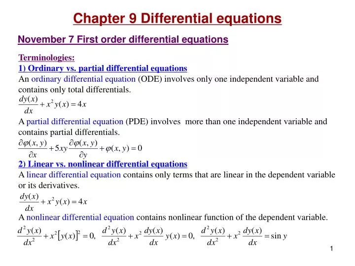
Chapter 9 Differential equations. November 7 First order differential equations. Terminologies: 1) Ordinary vs. partial differential equations An ordinary differential equation (ODE) involves only one independent variable and contains only total differentials.

E N D
Chapter 9 Differential equations November 7 First order differential equations Terminologies: 1) Ordinary vs. partial differential equations An ordinary differential equation (ODE) involves only one independent variable and contains only total differentials. A partial differential equation (PDE) involves more than one independent variable and contains partial differentials. 2) Linear vs. nonlinear differential equations A linear differential equation contains only terms that are linear in the dependent variable or its derivatives. A nonlinear differential equation contains nonlinear function of the dependent variable.
3) Order of a differential equation • The order of a differential equation is determined by the highest derivative in the equation. • 4) Homogeneous vs. inhomogeneous differential equations • A linear differential equation is homogeneous if every term contains the dependent variable or its derivatives. • A homogeneous differential equation can be written as where L is a linear differential operator. • A homogeneous differential equation always has a trivial solution y(x) = 0. • Superposition principle:If y1(x) and y2(x) are solutions to a linear homogeneous differential equation, then ay1(x) +by2(x) is a solution to the same equation.
An inhomogeneous differential equation has at least one term that contains no dependent variable. • Inhomogeneous equations are often called “driven” equations. They describe the response of the system to an external force. • The general solution to a linear inhomogeneous differential equation can be written as the sum of two parts:Here yh(x) is the general solution of the corresponding homogeneous equation, and yp(x) is any particular solution of the inhomogeneous equation.
9.2 First-order differential equations A first-order ordinary differential equation can be generally written as I. Separable variables If the equation has the form , then
II. Exact differential equations A first-order ordinary differential equation can be generally written as The differential is exactif we can find j (x, y) so that The solution of the differential equation is thus simply The condition for the differential to be exact is
Integrating factor Many times the differential is not exact. We can possibly multiply an integrating factor a(x,y) to both P and Q and make them exact:
Read: Chapter 9: 1-2 Homework: 9.2.2,9.2.3,9.2.4 Due: November 18
November 9, 11 Linear first order ODEs 9.2 First-order differential equations Linear first order ODEs: The general form of a linear first order ODE is All linear first order ODEs have a formulated solution.
Method of the variation of the constant in solving inhomogeneous ODEs:
Theorem: The solution of an inhomogeneous ODE is unique up to an arbitrary multiple of the solution of the corresponding homogeneous ODE. Linear dependence and Wronskian: Two solutions are linearly independent if has the only solution a=b=0. Otherwise the two solutions are linearly dependent. Theorem:A first order homogeneous ODE has only one linearly independent solution.
In general, for n functions the Wronskian is defined as
Theorem:A second order homogeneous ODE has at the most two linearly independent solutions. Theorem:An nth-order homogeneous ODE has at the most n linearly independent solutions. Corollary:The general solution of a second order homogeneous ODE is Corollary:The general solution of a second order inhomogeneous ODE is
Read: Chapter 9: 2 Homework: 9.2.11,9.2.13,9.2.14 Due: November 18
November 14 Separation of variables 9.3 Separation of variables (for partial deferential equations) Separation of variables is a technique which converts a PDE into a set of related ODEs. We look for the solution of the PDE that takes the form As an example let us consider the wave equation Let us first separate the space from the time dependence of the wave function. Now the lhs is a function of r while the rhs is a function of t. For them to be equal, they must each equals to a constant, called the constant of separation.
More about separation constants: A separation constant does not necessarily need to be exactly a constant. It can be a function and the differential equation may still be separable. Example:
Read: Chapter 9: 3 Homework: 9.3.4,9.3.9 Due: December 2
November 16,18 Series solution 9.4 Singular points Before we learn the series solution of differential equations, it is necessary to understand the singular points of differential equations. This is because singular points can possibly cause trouble when a series solution is attempted. We consider a point x = x0 for a second-order homogeneous differential equation • If P(x) and Q(x) are both finite at x = x0, then x = x0 is an ordinary point. • If either P(x) or Q(x) is infinite at x = x0, then x = x0 is a singular point. • If both (x-x0)P(x) and (x-x0)2Q(x) are finite as xx0, then x = x0 is a regular singular point. • If either (x-x0)P(x) or (x-x0)2Q(x) is infinite as xx0, then x = x0 is an irregular (essential) singular point. It can be shown that at an ordinary point or a regular singular point, it is possible to use the series solution approach. However, at an essential singular point the series solution method will most likely fail.
Singularity at infinity: We use variable z =1/x, and study the behaviors of the new coefficients of the differential equation as z0 .
9.5 Series solutions – Frobenius’ method The series solution method can be used to solve homogeneous ODEs that we have difficulty in solving them using other ways.
Question: What happens if we choose k = − m? Do we get another solution? The recurrence relation is then It does not work for j = 2m if m is an integer. Fuchs’ theorem: The Frobenius’ method can always obtain at least one power-series solution, provided we are expanding about a point that is an ordinary point or a regular singular point.If we attempt an expansion about an irregular or essential singularity, the method will most likely not work.
Read: Chapter 9: 4-5 Homework: 9.4.1,9.4.2,9.5.6(a),9.5.16 Due: December 2
November 28 A second solution 9.6 A second solution For a second-order homogeneous ODE we can always find a second linearly independent solution y2(x), provided that we have known a first solution y1(x) from other methods such as series solution. The Wronskian can be directly obtained from the differential equation without knowing its solutions. Solving a linear first-order ODE
Second order inhomogeneous differential equation: variation of constants Suppose a second-order homogeneous ODE has the solution y(x) = c1 y1(x)+ c2 y2(x), and the second-order inhomogeneous ODE has the solution y(x) = c1 y1(x)+c2 y2(x)+yp(x) = C1(x) y1(x)+ C2(x)y2(x), where C1(x)andC2(x)are going to be determined.
Read: Chapter 9: 6 Homework: 9.6.6,9.6.9,9.6.15,9.6.19 Due: December 9
November 30 Green’s function 9.7 Nonhomogeneous equation − Green’s function A nonhomogeneous linear differential equation can be written as L = Linear differential operator y(r) = Field to be found (response) f (r) = Source function (driving force) Because of the linearity of the equation, if f (r) can be decomposed into a series of function f (r) =Sifi(r), with each fi(r) causes a field of yi(r), i.e., then the solution of the original differential equation will be y1(r) + y2(r)+….We also know that any source function f (r) can be decomposed into a number of d functions by . Therefore if we can find the solution of the Green’s function the solution of the original differential equation will be Proof:
Notes to Green’s functions: • The Green’s function G(r, r') can be thought as the field distribution at r caused by a point source located at r'. • Since any source function is a sum of many point sources, the actual solution of a nonhomogeneous linear differential equation is a superposition of the Green’s function caused by each of the point sources. • The Green’s function is not one specific function. It is problem-specific, depending on the initial differential equation we are asked to solve. • Examples of Green’s functions: • Electrostatics.
Falling objects. An object is dropped at t =0. Though this seems to be cumbersome, it can be directly applied to solve an varying force problem. The power of Green’s function is then revealed:
z Z G(Y,Z;y',z') d (y-y',z-z') y Y z Z S(y,z) I(Y,Z) y Y Imaging process. How a camera works. The Green’s function for a point source is called a point-spread function, which is usually an Airy spot with some rings. The image is a superposition of the point-spread function, weighted by the source intensity. Though I do not know the actual differential equation involved.
Read: Chapter 9: 7 Homework: 9.7.5,6,15 Due: December 9
December 2 Helmholtz equation Example of Green’s functions: Helmholtz equation.
Quantum mechanical scattering: Neumann series solution and Born approximation
Read: Chapter 9: 7 No homework