Download

1 / 28
300 likes | 450 Views
LEVERAGE AND CAPITAL STRUCTURE. Business Risk and Financial Risk. Risk – the likely variability associated with expected revenue streams. The variations in the income stream can be attributed to: The firm’s exposure to business risk The firm’s decision to incur financial risk

E N D
Business Risk and Financial Risk • Risk – the likely variability associated with expected revenue streams. • The variations in the income stream can be attributed to: • The firm’s exposure to business risk • The firm’s decision to incur financial risk • Business Risk – the risk that comes from the nature of the firm’s operating activities. • Financial Risk – the risk that comes from the financial policy (i.e capital structure) of the firm.
Financial and Operating Leverage • Financial Leverage – the extent to which a firm relies on debt. The more debt financing a firm uses in its capital structure, the more financial leverage it employs. • Operating Leverage– the incurrence of fixed operating costs in the firm’s income stream.
Break-even Analysis • Objective – to determine the break-even quantity of output by studying the relationships among the firm’s cost structure, volume of output, and operating profit. • The break-even quantity of output results in an EBIT level = 0 • Some actual and potential applications of BEP include: • Capital expenditure analysis as a complementary technique to discounted cash flow evaluation models. • Pricing policy • Labor contract negotiations • Evaluation of cost structure • Financial decision making
Break-even Analysis • Essential elements of the break-even model: • Fixed cost – cost that do not vary in total amount as the sales volume or the quantity of output changes. Examples: • Administrative salaries • Depreciation • Insurance premiums • Property taxes • Rent • Variable cost – cost that tend to vary in total as output changes. VC are fixed per unit of output. Examples: • Direct materials • Direct Labor • Energy cost associated with production • Packaging • Freight-out • Sales commissions
Break-even Analysis • Semivariables costs (Semifixed cost) – cost that exhibit the joint characteristics of both FC and VC over different ranges of output. Examples: Salaries paid to production supervisors.
Finding Break-even Point • The break-even is just a simple adaptation of the firm’s income statement expressed as: • Profit (π) = Sales – (Total VC + Total FC) • 3 ways to find BEP: • Trial and Error • Select an arbitrary output level • Calculate the corresponding EBIT amount • When EBIT = 0, BEP has been found.
Finding Break-even Point • Contribution Margin Analysis • Contribution Margin = Unit Selling Price – Unit VC • BEP (units) = FC contribution margin per unit • Algebraic Analysis • QB = the break-even level of units sold P = the unit sales price F = the total FC for the period V = unit VC • Then, QB = F P – V
Finding Break-even Point Example: Mutiara Corporation (MC) manufactures a complete line of women’s dress. It sells each dress for RM 30. The variable cost for this dress is 70% of sales. Mutiara Corporation; incurs fixed costs of RM 360,000, how many dress must MC sell to breakeven?
Finding Break-even Point Solutions: *unit variable cost (VC) = 70% x RM 30 = RM 21 QB = F P – V = RM 360 000 = 40 000 unit RM 30 – RM 21
Finding Break-even Point • The BEP in sales dollars: • S* = F 1 – VC S Example: Sales $ 300 000 (-) Total VC 180 000 Revenue before FC 120 000 (-) Total FC 100 000 EBIT $ 20 000
Finding Break-even Point Solutions: S* = F = $ 100 000 1 – VC 1 – $ 180 000 S $ 300 000 = $ 100 000 1 – 0.60 = $ 250 000
Degree of Operating Leverage • Degree of Operating Leverage from the base = % change in EBIT sales level (DOLs) % change in Sales • DOLs = Q (P – V) Q (P – V) – F • DOLs = revenue before FC = S – VC EBIT S – VC – F
Degree of Operating Leverage Example: Avitar Corporation manufactures a line of computer memory expansion boards used in microcomputers. The average selling price of its finished product is $175 per unit. The variable cost for these same units is $115. Avitar incurs fixed costs of $650,000 per year. Avitar estimates the sales in next year will be 20,000 units. What is Avitar expected degree of operating leverage?
Degree of Operating Leverage Solutions: DOLs = Q (P – V) Q (P – V) – F = 20 000 ($ 175 – $ 115) [20 000 ($ 175 – $ 115)] – $ 650 000 = 2.1818 times
Degree of Financial Leverage • DFL = % change in EPS > 1 % change in EBIT • DFLEBIT = EBIT EBIT – I * I = interest expense
Degree of Financial Leverage Example: Sales $ 600,000 (-) total VC $ 200,000 Revenue before FC $ 400,000 (-) total FC $ 200,000 EBIT $ 200,000 (-) interest expenses $ 50,000 EBT $ 150,000 Taxes (34%) $ 51,000 Net Income (EAT) $ 99,000
Degree of Financial Leverage Solutions: What is the degree of financial leverage? DFLEBIT = EBIT EBIT – I = $ 200 000 $ 200 000 – $ 50 000 = 1.33 times
Combination of Operating and Financial Leverage • DCL = % change in EPS % change in Sales • DCLs = (DOLs) x (DFLEBIT) • DCLs = Q (P – V) Q (P – V) – F – I
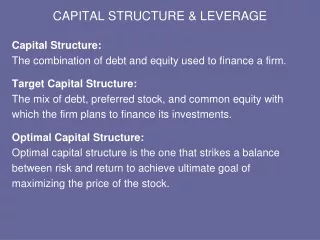
Planning the Firm’s Financing Mix • Financial Structure – the mix of all funds source that appear on the right side of the balance sheet. • Capital Structure – the mix of long term sources of funds used by the firm. Basically, this concept omits short-term liabilities. • Financial Structure Design – the management activity of seeking the proper mix of all financing components in order to minimize the cost of raising a given of funds. • Optimal Capital Structure – the unique capital structure that minimizes the firm’s composite cost of long term capital.
Planning the Firm’s Financing Mix • EBIT-EPS indifference point – the level of EBIT that will equate EPS between two difference financing plans. EPS: Stock Plan EPS: Bond Plan (EBIT – I) (1 – t) – P = (EBIT – I) (1 – t) – P Ss Sb * EBIT = earning before interest and taxes I = interest expenses t = firm income tax rate P = preferred dividend paid Ss = the number of common s/o under the stock plan Sb = the number of common s/o under the bond plan
Planning the Firm’s Financing Mix • Projected Income Statement Alternative 1 Alternative 2 EBIT XXXXXX XXXXXX (-) Interest XXXXX XXXXX EBT XXXXXX XXXXXX (-) Taxes XXXXX XXXXX Net Income XXXXXX XXXXXX Shares XXXXXXX XXXXXXX EPS* XXX XXX *EPS = Net Income Shares Outstanding
Planning the Firm’s Financing Mix Example: ING Berhad is financed entirely with 800,000 shares of common stock priced at RM 5 per unit and RM 1,000,000 worth of debt (8% 10 years bond). The company plans to raise an additional RM 2,000,000 to finance new project and considering two alternatives; Alternative 1: 200,000 new common shares sold to the public Alternative 2: Issue 10% bond Projected level of EBIT is at approximately RM 2,000,000. Corporate tax rate is 28%.
Planning the Firm’s Financing Mix Solutions: • Calculate the indifference level of EBIT between two alternatives. * Plan Stock (alternative 1) = Interest on bond = (1,000,000 x 8% = RM 80,000) Unit shares = 800,000 + 200,000 = 1,000,000 *Plan Bond (alternative 2) = Interest on bond = RM 80,000 + (RM 2,000,000 x 10% = RM 280,000) Unit shares = 800,000
Planning the Firm’s Financing Mix Plan Stock Plan Bond (EBIT – I) (1 – t) – P = (EBIT – I) (1 – t) – P Ss Sb (EBIT – 80,000) (1 – 0.28) – 0 = (EBIT – 280,000) (1 – 0.28) - 0 1,000,000 800,000 0.72 EBIT – RM 57,600 = 0.72 EBIT – RM 201,600 1,000,000 800,000 576,000 EBIT – RM 46,080,000,000 = 720,000 EBIT – RM 201,600,000,000 – 144,000 EBIT = – RM 155,520,000,000 EBIT = RM 1,080,000
Planning the Firm’s Financing Mix • Prepare the projected income statement that proves EPS will be the same regardless of the plan chosen at the EBIT level found in question (i) Alternative 1 Alternative 2 EBIT RM 1,080,000 RM 1,080,000 (-) Interest 80,000 280,000 EBT 1,000,000 800,000 (-) Taxes (28%) 280,000 224,000 Net Income 720,000 576,000 Shares 1,000,000 800,000 EPS* 0.72 0.72 *EPS = Net Income Shares Outstanding
Planning the Firm’s Financing Mix • Which plan will provide the highest EPS for the EBIT projected level? Alternative 1 Alternative 2 EBIT RM 2,000,000 RM 2,000,000 (-) Interest 80,000 280,000 EBT 1,920,000 1,720,000 (-) Taxes (28%) 537,600 481,600 Net Income 1,382,400 1,238,400 Shares 1,000,000 800,000 EPS* 1.3824 1.548 *EPS = Net Income Shares Outstanding