Download
1 / 36
360 likes | 502 Views
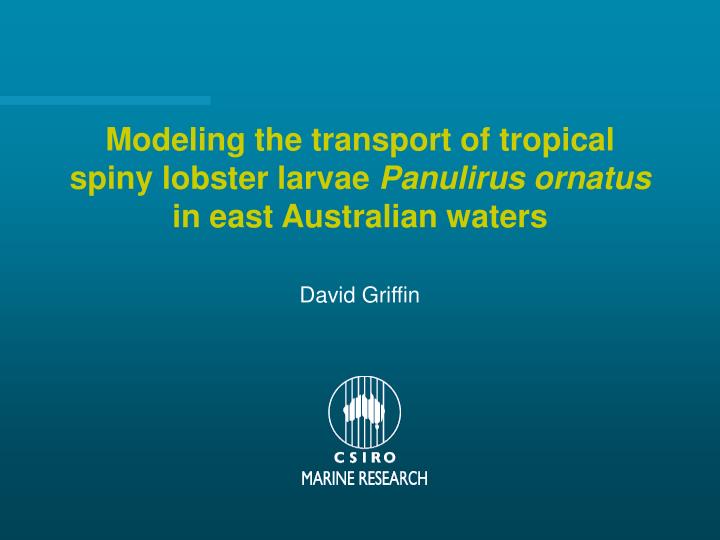
Modeling the transport of tropical spiny lobster larvae Panulirus ornatus in east Australian waters. David Griffin. Larval transport – why study it?. To find out what adult population your region depends on for recruits To find out which regions (if any) depend on yours for recruits.

E N D
Modeling the transport of tropical spiny lobster larvae Panulirus ornatus in east Australian waters David Griffin
Larval transport – why study it? • To find out what adult population your region depends on for recruits • To find out which regions (if any) depend on yours for recruits
Larval transport – how to study it? • Much insight into the dispersal of larvae has been gained by sampling at sea • This has revealed where larvae are found – region, depth, etc • But it does not provide the answers we need • computer simulation an important additional approach • We’ve used an individual-based transport model, using estimates of ocean currents derived from satellite measurements of sealevel.
Technical details • NCEP/NCAR reanalysis winds. Surface drift 2%*u10. Time dependent Ekman layer h=50m, r=0.0002m/s • Topex/Poseidon, ERS 1&2 and tidegauges. Cyclostrophic velocity fields. • Mean velocity from ACOM3.1. New model (10km*10km) nearly finished. • Random walk at 2 length and time scales • Integration by 4th order Runge-Kutta. • U=0 at coast, ‘beaching’ larvae returned. • Metamorphosis on encountering the 100m isobath • Pueruli swim shoreward at 0.1m/s for 30days max.
How realistic are these results? • Important: the model does not include all processes affecting larval transport – only advection (and not even all advective processes) • Missing details of: shelf circulation, vertical migration, vertical shear, metamorphosis, swimming • completely missing: spatio-temporal variations of mortality from starvation and predation • So it would be surprising if details of the simulations, eg location of larvae at the time of a cruise, or settlement rates at some point, matched observations
So what have we learnt? • Larvae from the Australian and PNG stocks mix in the Coral Sea gyre • This stock of P Ornatus appears to be self-supporting • Variability of winds (especially cyclones), and currents means larval transport varies greatly from year to year • Nevertheless, the basic picture is determined by the mean positions of the South Equatorial, Hiri and East Australian currents. Larvae hatching south of the SEC bifurcation are less likely to recruit north of it, and hence are, to some extent, a ‘sink’ population.
What next? • Improve estimates of biological parameters (hatch times and locations, variability of mortality of all larval stages, puerulus behaviour) • Enlarge model domain while increasing accuracy and resolution, use hydrodynamic model instead of geostrophic currents