CHAPTER TEN Aggregate Demand I

1. CHAPTER TEN Aggregate Demand I

2. The Great Depression caused many economists to question the validity of classical economic theory (from Chapters 3-6). They believed they needed a new model to explain such a pervasive economic downturn and to suggest that government policies might ease some of the economic hardship that society was experiencing. In 1936, John Maynard Keynes wrote The General Theory of Employment, Interest and Money. In it, he proposed a new way to analyze the economy, which he presented as an alternative to the classical theory. Keynes proposed that low aggregate demand is responsible for the low income and high unemployment that characterize economic downturns. He criticized the notion that aggregate supply alone determines national income.

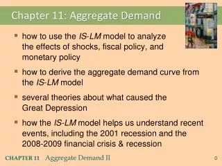
3. This chapter: Aggregate Demand 1. The goods market and the IS curve 2. The money market and the LM curve 3. The short-run equilibrium

4. The Keynesian Model

5. Background on the Model The basic textbook Keynesian model: an elaboration and extension of the ‘classical theory’. Its variables velocity of money and ‘sticky’ prices reflects Keynes’ belief that the Classical model’s shortcomings arose from its overly-strict assumptions of constant velocity and highly flexible wages and prices.

6. The Keynesian model - shows what causes the aggregate demand curve to shift. Price Level, P AD'' AD' SRAS AD Income, Output, Y Y* Y*' Y*'' In the short run, when the price level is fixed, shifts in the aggregate demand curve lead to changes in national income, Y. The IS-LM model = the leading interpretation of Keynes’ work. The goal of the model: to show what determines national income for any given price level.

7. The model of aggregate demand (AD) can be split into two parts: - IS (“investment” and “saving”)model of the ‘goods market’ - LM (“liquidity” and “money”) model of the ‘money market’.

8. The Goods Market and the IS Curve The IS curve (which stands for investment and saving) plots the relationship between the interest rate and the level of incomethat arises in the market for goods and services. The Money Market and the LM Curve The LM curve (which stands for liquidity and money) plots the relationship between the interest rate and the level of income that arises in the money market. The variable that links the two parts of the IS-LM model: the interest rate (it influences both investment and money demand).

9. 1. The Goods Market and the IS Curve In the General Theory of Money, Interest and Employment (1936), Keynes proposed: an economy’s total income was, in the short run, determined largely by the desire to spend by households, firms and the government. Thus, the problem during recessions and depressions, according to Keynes, was inadequate spending. How to model this insight? - The Keynesian Cross

10. The Keynesian Cross Actual expenditure = the amount households, firms and the government spend on goods and services (GDP). Planned expenditure = the amount households, firms and the government would like to spend on goods and services. The economy is in equilibrium when: Actual Expenditure = Planned Expenditure or Y=E Actual Expenditure, Y=E Expenditure, E Planned Expenditure, E = C + I + G Income, Output, Y Y1 Y2 Y*

11. Question: How does the economy get to this equilibrium? - Inventories play an important role in the adjustment process. Actual Expenditure, Y=E Expenditure, E Planned Expenditure, E = C + I + G Income, Output, Y Y1 Y2 Y*

12. Let’s see how changes in government purchases affect the economy. Actual Expenditure, Y=E Expenditure, E B Planned Expenditure, E = C + I + G A DG Income, Output, Y Y1 Y* An increase in government purchases of ΔG raises planned expenditure by that amount for any given level of income. The equilibrium moves from A to B and income rises. Note: the increase in income Y exceeds the increase in government purchases ΔG. Thus, fiscal policy has a multiplied effect on income.

13. Fiscal Policy and the Multiplier If government spending were to increase by $1, then you might expect equilibrium output (Y) to also rise by $1. But it doesn’t! The multiplier shows that the change in demand for output (Y) will be larger than the initial change in spending. Here’s why: When there is an increase in government spending (G), income rises by G as well. The increase in income will raise consumption by MPC  G, where MPC is the marginal propensity to consume. The increase in consumption raises expenditure and income again. The second increase in income of MPC  G again raises consumption, this time by MPC  (MPC  G), which again raises income and so on. So, the multiplier process helps explain fluctuations in the demand for output. For example, if something in the economy decreases investment spending, then people whose incomes have decreased will spend less, thereby driving equilibrium demand down even further.

14. The government-purchases multiplier: DY/DG = 1 + MPC + MPC2 + MPC3 + … DY/DG = 1 / 1 - MPC The tax multiplier: DY/DT = - MPC / (1 - MPC)

15. The Interest Rate, Investment and the IS Curve • Let’s now relax the assumption that the level of planned investment is fixed. • - We write the level of planned investment as: I = I (r). • The investment function - downward-sloping (it shows the inverse relationship between investment and the interest rate) • The IS curve summarizes the relationship between the interest rate and the level of income. It is downward-sloping. • The IS curve combines: • the interaction between I and r expressed by the investment function • the interaction between I and Y demonstrated by the Keynesian cross.

16. Deriving the IS Curve An increase in the interest rate (in graph a), lowers planned investment, which shifts planned expenditure downward (in graph b) and lowers income (in graph c). (b) The Keynesian Cross E Y=E Planned Expenditure, E = C + I + G Income, Output, Y (a) (c) r r The Investment Function The IS Curve I(r) IS Income, Output, Y Investment, I

17. An increase in government purchases The Keynesian Cross How fiscal policy shifts the IS curve? E Y=E Planned Expenditure, E = C + I + G An increase in government purchases or a decrease in taxes - IS curve shifts outward. A decrease in government purchases or an increase in taxes - IS curve shifts inward. Income, Output, Y r The IS Curve IS2 IS1 Income, Output, Y

18. Summary • The IS curve shows the combinations of the interest rate and the level of income that are consistent with equilibrium in the market for goods and services. • The IS curve is drawn for a given fiscal policy. • Changes in fiscal policy that raise the demand for goods and services shift the IS curve to the right. • Changes in fiscal policy that reduce the demand for goods and services shift the IS curve to the left.

19. r Supply Demand, L (r) M/P M/P 2. The Money Market & LM Curve LM curve = the relationship between the interest rate and the level of income that arises in the market for money balances The theory of liquidity preference - how the interest rate is determined in the short run The supply of real money balances - vertical The demand for real money balances - downward sloping The supply and demand for real money balances determine the equilibrium interest rate.

20. L(r) = M/P Money Demand Real Money Balances equals Money Market Equilibrium

21. Supply' r Supply Demand, L (r,Y) M/P M/P A Reduction in the Money Supply: -M/P Since the price level is fixed, a reduction in the money supply reduces the supply of real balances. Notice the equilibrium interest rate rose.

22. Money Demand (M/P)d = L (r,Y) The quantity of real money balances demanded is negatively related to the interest rate (because r is the opportunity cost of holding money) and positively related to income (because of transactions demand).

23. r2 r1 r Supply L (r,Y)' L (r,Y) M/P M/P Deriving the LM Curve r LM Y An increase in income raises money demand, which increases the interest rate; this is called an increase in transactions demand for money. The LM curve summarizes these changes in the money market equilibrium.

24. LM' Supply' Supply r2 r2 M´/P M/P Shifting the LM Curve r r LM r1 r1 L (r,Y) M/P Y A contraction in the money supply raises the interest rate that equilibrates the money market. Why? Because a higher interest rate is needed to convince people to hold a smaller quantity of real balances. As a result of the decrease in the money supply, the LM shifts upward.

25. Summary • The LM curve shows the combinations of the interest rate and the level of income that are consistent with equilibrium in the market for real money balances. • The LM curve is drawn for a given supply of real money balances • Decreases in the supply of real money balances shift the LM curve upward • Increases in the supply of real money balances shift the LM curve downward

26. IS r LM(P0) r0 Y Y0 The IS-LM Model of AD The IS curve/equation Y= C (Y-T) + I(r) + G The LM curve/equation M/P = L(r, Y) The intersection of the IS and LM curves represents simultaneous equilibrium in the market for goods and services and in the market for real money balances for given values of government spending, taxes, the money supply, and the price level.

27. Key Concepts of Ch. 10 IS-LM Model IS Curve LM Curve Keynesian cross Government-purchases multiplier Tax multiplier Theory of liquidity preference