Download
1 / 66
660 likes | 848 Views
Aggregate Demand. Up to this point we have looked at the basic concepts of RGDP, unemployment and inflation. This is good because we have to have a solid understanding of these ideas.

E N D
Up to this point we have looked at the basic concepts of RGDP, unemployment and inflation. This is good because we have to have a solid understanding of these ideas. Next we build a model of the economy that we will use to help us understand why RGDP, unemployment, inflation and other related concepts change. If we can understand why changes happen, then perhaps performance of these macroeconomic variables can be managed. The model we will work with is called the model of Aggregate Demand (AD) and Aggregate Supply (AS). For a while our focus will be on Ad and AS separately, then we will bring the two parts together. Our model is about AD and AS interacting to “produce” the results in the economy. But, we look at the mechanics of each part first.
Aggregate Demand Aggregate demand refers to the amount of real output, RGDP, that buyers collectively desire to purchase at each possible price level. Remember from our earlier work that the buyers referred to here are in 1 of 4 groups: Households undertaking consumption (C), Businesses undertaking investment (I), Governments undertaking government purchases (G), and The rest of the world undertaking net exports (Xn)(the buying of goods made in US, net of any items purchased here but made in other countries).
AD in a graph Price level AD RGDP
Downward slope of AD curve Note the downward slope of the AD curve as you look at the curve from left to right. The relationship between the price level and the amount of RGDP desired is said to be inverse. Now we want to give this idea economic meaning. There are 3 reasons for the downward sloping AD curve. 1) Real balance or real wealth effect – as the price level rises the purchasing power of people’s assets such as savings accounts or bonds declines. Folks are poorer and thus causes households to reduce C and save a bit so they can afford essentials in the future.
Downward slope of AD curve 2) Interest rate effect – (we see this idea more later) as the price level rises you and I demand more money (the gallon of milk we buy for 2.00 goes up to, say about two fifty, and so we need more money to make our transactions). With a given money supply, a higher money demand makes the interest rate rise and thus consumption and investment fall. 3) Foreign purchases effect – as the price level domestically rises (assuming the rate does not change in other countries), it becomes increasingly difficult for foreigners to buy our goods and we want more of their goods and thus net exports fall.
Shift AD curve The AD line can also shift left or right. What things make the AD line shift (we call these things demand shifters or determinants of AD)? Remember we said Households undertake consumption (C), Businesses undertake investment (I), Governments undertake government purchases (G), and The rest of the world undertakes net exports (Xn)(the buying of goods made in US, net of any items purchased here but made in other countries). Anything that changes these components (except for a price level change) will shift the AD curve.
Consumption The greater the wealth, w, the greater will consumption be and AD shifts right. expc, or consumer expectations about the future, has an influence on C. The more confident about the future consumers are, the more will consumption spending be now and AD shifts right. The higher the level of household debt, HD, the more consumption can occur and AD shifts to the right. If taxesc (= taxes on households) rise then consumption will fall. In fact if taxesc go up by X the C falls by MPC times X and the AD curve shifts to the left. (The reverse of each factor follows the same basic pattern.)
Investment I = I(amo, bt, tc, expb, i), where I = investment plans, amo = Acquisition, maintenance, and operating costs, bt = Business taxes, tc = technological change, expb= expectations business have about the future, and i= the interest rate. If amo goes up I goes down and AD shifts left. If bt goes up I goes down and AD shifts left. If tc goes up I goes up and AD shifts right. The higher the business expectation about the future the more investment will be today and AD shifts right. A higher interest rate means it is more costly to invest, so less will happen and AD will shift to the left.
Government Spending and Net Exports G = G(politics), so government spending is largely determined in the political arena. An increase in G shifts AD right. Xn= Xn(for, e) where Xn= net exports and for = the health of foreign economies and e = relative strength of dollar against other currencies. If foreign economies get better then Xn rises and AD shifts right. If the dollar appreciates more exports from US are more difficult for foreigners and it is easier for us to make imports. Xn falls and the AD shifts to the left.
AD shifting and the multiplier Price level AD1 AD2 RGDP
AD shifting and the multiplier On the previous slide I have AD1, AD2 and an AD curve between the 2. When we look back at all the items that can shift the AD, if we get a shift from one of these items then the first shift is from AD1 to the dashed line. Recall that the multiplier concept was about an initial change in spending is transformed into a larger change in RGDP. Here this means after the initial change due to a demand shifter change, the multiplier will kick in and shift the AD curve even more.
Aggregate Supply The AS is the part of our national economy model where the production side is studied.
An Analogy and a definition Which blade cuts the paper when you use a pair of scissors on the paper? The answer is that you need both to cut the paper. Up to now in our theory about the national economy we have talked about aggregate demand, AD. But, just like we need both blades in the scissors, we also have to build in aggregate supply into our theory. Aggregate Supply AS is about the relationship between the price level and the amount of real domestic output (RGDP) that firms in the economy produce.
Recall an earlier story Please recall our earlier work about a single firm and its production when prices were sticky and when they could freely adjust. With sticky prices we saw a horizontal supply and with flexible prices we saw a vertical supply. In the larger, full economy we recall this earlier story and build on it. In macro we will think about three scenarios: 1) Input prices and output prices are fixed, or are sticky, 2) Input prices are fixed but output prices can change, and 3) Both input prices and output prices can change. Let’s explore each of these scenarios next.
The Immediate Short Run Fact about our economy: 75% of a typical firm’s costs are wage and salary and these are fixed either by contract (like for me) or there is an implicit understanding that wages are negotiated only every so often (maybe yearly). A good deal of input prices are fixed in this time frame. Price level P1 ASISR RGDP
The Immediate Short Run Also in the immediate short run output prices are fixed. Firms print up menus and price lists and in the very short term they stick with these prices. So, the immediate short run is anywhere from a few days to a few months. The more important point is that it is that period of time when both input prices and output prices are fixed (sticky!). Hey, try not to be confused by input prices and output prices. Example: Say the output is pizza. The output price is the price of the cooked pizza. What are the inputs to making pizza? The dough, sauce and other ingredients are inputs that will have prices, as will the labor that is making the pizza (and the price of labor is often called the wage!).
The Immediate Short Run Note that the level of output in this immediate short term will depend on aggregate demand and the RGDP level that corresponds to full employment will only occur if demand is AD Full. In other words the full employment level of output is not guaranteed in the economy. Price level AD Full AD Low AD High P1 ASISR Full Low RGDP High
Short Run P The AS has an upward slope to it as we view it from left to right. This means the price level and the level of RGDP firms will offer for sale is positively, or directly, related. AS P1 P2 RGDP1 RGDP2 RGDP
Short Run Note that the short run is defined here as the time frame in which input prices are fixed but output prices can change. Higher (lower) output prices with fixed input prices means profits would be higher (lower) and this is the incentive (disincentive) firms need to increase (decrease) real output. On the last screen you can see that at low levels of RGDP the AS is somewhat flat and as the level of RGDP rises the curve is becomes steeper. Let’s look at this next.
Per Unit Production Cost In order to see the points about AS we need to think about the following ratio: Total input cost/units of output. This ratio is the per unit production cost (on average) of output. Ultimately the price per unit of output has to cover this or firms would not be able to produce because they wouldn’t be making any profit. The AS is a curve showing what price levels have to be to get the various levels of output produced. Now, if more units of output are made, additional inputs are needed (but remember the short run has the input prices fixed!).
Per unit production cost When output is already low, below the full employment level, this means many resources are underutilized. To add output resources that are idle get put back to work and the ratio of input cost to output does not change much. So the price level does not have to expand much to get more output. With the higher price level firms have an incentive to produce more. Now, when output is already at the full employment level of output or above, additional output is that much harder to come by. Adding inputs, when a great deal of output is already being made does not yield as much output as before and thus per unit costs rise. In order to get the additions, the price level would have to really jump to get the additional output.
Long run Given a state of technology and resource endowments the ASLRis shown as one level of RGDP. This is the full employment level of output in the economy.Since it is a vertical line, we see that if the price level should change the quantity supplied in the long run will not change. P ASLR P2 P1 RGDP RGDP1
Long Run The long run is defined as the time frame in which both input prices and output prices can change. Say that the economy is really producing a great deal of output. When the economy is operating at a high level workers are often putting in a lot of overtime because there are few excess workers and other resources. After a while workers and other resource owners conclude that input prices need to adjust because of this work pattern. Higher output prices resulting from high levels of output soon get matched with higher input prices. Output then stays at the potential level in the economy.
Summary up to Now The immediate short run aggregate supply is referred to as ASISR and is the result of both input and output prices being fixed. The short run aggregate supply is referred to as AS and is the result of input prices being fixed but output prices as being flexible. The long run aggregate supply is referred to as ASLR and is the result of both input and output prices being flexible. The authors note that a great deal of our time will focus on the short run and unless otherwise stated that will be the context of the discussion of aggregate supply for now. The reason for this is because business cycles are thought to have the same conditions as under the short run – namely flexible output prices, inflexible input prices.
There are 3 kinds of people in the world. There are those who can count and those who can’t ! Shifting AS The AS supply curve can shift if we have a change in 2) productivity, 3) business taxes and subsidies, and 4) government regulation. Let’s look at each idea here next. If productivity grows then firms can make available for sale a greater number of goods available for sale at each price level – The AS shifts to the right. When business taxes grow, or when subsidies fall, firms have to pay out a greater amount from the price level they receive and therefore they keep less. The fact that they keep less makes them more reluctant to supply and thus AS shifts to the left. Government regulation is usually costly for the firm to cover and so more regulations reduce AS and this means the curve shifts to the left.
Shifting AS The AS supply curve can shift if we have a change in 1) Input prices – WAIT A MINUTE – before we said input prices were fixed in the short run! What is up? The real story is that as the long run is approached input prices change and this will cause a shift in the short run AS. Plus there are shocks on the supply side that cause inputs prices to change. If input or resources prices rise, then per unit production costs rise and thus at the same price level firms in total would reduce output and AS would shift to the left. Note some inputs in US economy actually come from other countries. So, if the dollar becomes weaker foreign inputs get more expensive because we need more dollars to get a unit of foreign currency.
AD and AS together Here we put Aggregate Supply in the short run and Aggregate Demand together and use the model to help use understand the actual performance of the macroeconomic system.
Equilibrium in SR P AD1 AS1 P1 RGDP RGDP1
Equilibrium On the previous slide we have the AD curve cross the AS. This is our usual starting point. Note the price level is determined at this intersection and the level of RGDP is determined at this point. The economy would stay at this point in the short run and there we observe price level P1 and RGDP level RGDP1 in the economy if every thing else stayed the same. The real world, though, is one of change and things will not stay the same. Let’s see how our model works here.
Rise in AD P AS P2 P1 AD2 AD1 RGDP RGDP1 RGDP2
Rise in AD Say the AD rises (remember why AD could shift to the right? – maybe G increases or I increase, or we have seen many other reasons) With the AD rising along the given AS curve the tendency is for the price level to rise. This higher price will 1) Encourage movement along the AS so more output is produced, but 2) Encourage movement along the new AD, but this a decline back to where the AS and new AD meet. The higher price level here is inflation and since demand growth caused it we would say there is demand pull inflation.
Rise in AD If RGDP1 a few slides back was the full employment level of output, then when AD shifts right and we end up at RGDP2, the difference RGDP2 minus RGDP1 would be called a positive, or inflationary, GDP gap. Note: from our discussion of the multiplier, the amount the AD curve shifted would be the full multiplier impact of a change in C, I, G or X. But, when the price level changes some of this multiplier amount is choked off.
Fall in AD P AD1 AS1 P1 AD2 P2 RGDP2 RGDP RGDP1
Fall in AD AD can fall for many reasons we have covered. Our model would suggest that not only would RGDP fall, but the price level would fall as well. RGDP would fall less than the shift in AD because the lower price level would reverse some of the decline in AD.
Decrease in AS P AS2 AD1 AS1 P1 RGDP RGDP1
Decrease in AS Back in the 1970’s, and again in the 2000’s, in the US we had the “oil supply shocks” which put pressure on production because oil, or its by-products, is used in many production processes. This shifted the AS to the left. With AS shifting left the price level rose and RGDP fell. The higher price level is inflation and in this case is called cost push inflation due to higher costs of production. The decline in RGDP would be called a recession. Note along the new AS the higher price has been “ratcheted up.”
AD and AS together Here we put Aggregate Supply and Demand together and use the model to help use understand the actual performance of the macroeconomic system.
I would like to use another analogy here – this one from the world of medicine. Have you every had a sinus infection? No fun! Can you live with a sinus infection and have the infection go away without any hands on intervention from a doctor? The answer is yes, but why would you want to in modern America? Please think about this! Sometimes we may want a hands off approach.
A point about the method When we talked about Aggregate Supply we made it a point to distinguish between the short run and the long run. We are always in a short run and are moving toward a long run. In AD/AS graphs we use from here out focus your attention on the AD - SRAS intersection and if this happens at a place other than where LRAS, then an automatic adjustment will happen in the economy as we talked about during our discussion about SRAS. The adjust will include a shift of the SRAS curve.
Equilibrium P LRAS AD1 SRAS1 P1 RGDP RGDP1
Equilibrium On the previous slide we have the AD curve cross the SRAS exactly where the SRAS crosses the LRAS. This is our usual starting point. Note the price level is determined at this intersection and the level of RGDP is determined at this point. The economy would stay at this point and then we observe price level P1 and RGDP level RGDP1 in the economy if every thing else stayed the same. The real world, though, is one of change and things will not stay the same. Let’s see how our model works here.
Rise in AD P LRAS AD1 SRAS1 P2 P1 AD2 RGDP1 RGDP2 RGDP
Rise in AD Say that AD rises. Since at P1 the AS is at RGDP1 and the AD is more, the national economy shortage will pull the price level up and firms will follow along the SRAS by adjusting input usage. The short term impact is to have the price level rise and the level of RGDP rise. The increase in the price level is called inflation. We have a demand theory of inflation. If demand rises the level of prices will rise. This is a demand pull theory of inflation.
Rise in AD The distance RGDP2 - RGDP1 is called an expansionary or positive GDP gap. It is the gap by which the economy has expanded above the natural pace of the economy. The expansionary gap will naturally go away in the long run if nothing else changes. The way this will happen is the input prices will eventually rise because resources are being worked hard. With higher input prices the SRAS shifts to SRAS2 and the economy is back at the natural level of output, although at a higher price level. We see this on the next slide. Again, the time frame of the adjustment may lead policy makers to take action before the long run natural mechanism can take place.
In the long run an increase in AD only changes the price level (to P3). Rise in AD P LRAS SRAS2 P3 AD1 SRAS1 P2 P1 AD2 RGDP1 RGDP2 RGDP
Fall in SRAS P LRAS SRAS2 AD1 SRAS1 P1 RGDP RGDP1 47
Fall in SRAS On the previous slide say we have a oil prices spike up high or some other widely used input has an increase in price. This input price rise can cause SRAS to shift left. We would then have inflation with reduced output. The reduced output would be recognized as a recession with more unemployment and the higher price would be inflation. If nothing is done from a policy perspective the recession and unemployment would eventually lead to lower input prices as inputs simply seek employment. Eventually the SRAS would shift back to SRAS1. But, if this takes a long time the unemployment may cause policy makers to want to increase AD without waiting for SRAS to shift out. This would cure the unemployment, but would mean even more inflation. (see this on the next slide)
Fall in SRAS P LRAS SRAS2 AD1 SRAS1 P1 RGDP RGDP1 49
Fall in AD P LRAS AD1 SRAS1 P1 AD2 P2 RGDP2 RGDP RGDP1