Download
1 / 23
240 likes | 1.16k Views
Chapter 2 - Map Projection. 9-1-2004 Week 1. Introduction. Same coordinate system is used on a same “ View ” of ArcView or same “ Data Frame ” in ArcMap. Projection - converting digital map from longitude/latitude to two-dimension coordinate system.

E N D
Chapter 2 - Map Projection 9-1-2004 Week 1
Introduction • Same coordinate system is used on a same “View” of ArcView or same “Data Frame” in ArcMap. • Projection - converting digital map from longitude/latitude to two-dimension coordinate system. • Re-projection - converting from one coordinate system to another
Size and Shape of the Earth • Shape of the Earth is called “geoid” • The sciences of earth measurement is called “Geodesy” • “ellipsoid” - reference to the Earth shape. b=semiminor axis (polar radius) f = (a-b)/a - flattening 1/298.26 for GRS1980, and 1/294.98 for Clarke 1866 a = semimajor axis (equatorial radius) The geoid bulges at the North Pole and is depressed at the South Pole
Geographic Grid • The location reference system for spatial features on the Earth’s surface, consisting of Meridians and Parallels. • Meridians - lines of longitude for E-W direction from Greenwich (Prime Meridian) • Parallels - line of latitude for N-S direction • North and East are positive for lat. and long. such as Cookeville is in (-85.51, 36.17).
DMS and DD (sexagesimal scale) • Longitude/Latitude can be measured in DMS or DD, • For example in downtown Cookeville, a point with (-85.51, 36.17) which is in DD. To convert DD to DMS, we will have to do several steps: for example, to convert -85.51 to DMS, • 0.51 * 60 = 30.6, this add 30 to minute and leave 0.6. • 0.6 * 60 = 36, this add 36 to seconds. Thus, the longitude is (-85o30’36”)
Exercise - convert New York City’s DMS to DD • New York City’s La Guardia Airport is located at (73o54’,40o46’). Convert this DMS to DD.
Exercise - convert New York City’s DMS to DD • New York City’s La Guardia Airport is located at (73o54’,40o46’). Convert this DMS to DD. • 54/60 = 0.9 and 46/60 = 0.77 • (73.90, 40.77) is the answer.
Length of Parallels/Angular/Great Circle • Length of parallels = cos() * length of equator • Meridians and parallels intersect at right angles. • Loxodrome – meridians, parallels and equator all have constant compass bearing. • Great circle arc – shortest distance between 2 points on earth, formed by passing a plane through the center of the sphere. • All meridians and equator are great circle. • Small Circle – circles on the grid are not great circle. Parallels of latitude of small circle (except equator). • Travel along N-S is the shortest, but not E-W (except along equator) • Azimuth – angel between great circle and meridian (fig 2.10)
Measure Distance on a Spherical Surface • cos D = sin a * sin b + cos a * cos b * cos c • where D is the distance between A and B in degrees • a is the latitude of A, b is the latitude of B and c is the difference in longitude between A and B. • Multiply D by by the length of one degree at the equator,which is 69.17 miles. For example: • Between Cookeville and New York City, we have a = 36.17, b=40.77, and c = -85.51 - (-73.90) = - 11.61 • cos D = sin36.17 * sin 40.77 + cos 36.17 * cos 40.77 * cos (-11.61) = 0.988, cos-1 0.988 = 8.885 • Distance = 8.885 * 69.17 = 615 miles
Projection – to represent the earth as a reduced model of reality • Transformation of the spherical surface to a plane surface. Graticule – meridians and parallels on a plane surface. • Projection Process (fig 2.12) • Best fit (earth geoid) • Reference ellipsoid • Generating globe • Map projection (2D surface)
Scale • Map Scale = map distance / earth distance • RF (representative fraction) – such as 1:25,000, 1:50,000… • Compute the scale with 10-in radius globe • Scale Bar, Verbal Scale (1 in = 2 miles) • Determine scale of “1 inch to 4 miles • Scale problem – distance between two points is 5 mile, what is the scale of a map on which the points is 3.168 inches apart?
Map projections • Distortion caused by tearing, shearing and compression from 3D to 2D. • For a large scale map, distortion is not a major problem. However, the mapped is larger, then distortion will occur. • Conformal - preserves local shapes • Equivalent - preserves size • Equidistant - maintain consistency of scale for certain distance • Azimuthal - retains accurate direction • Conformal and Equivalent - mutually exclusive, otherwise a map projection can have more than one preserved property
Projections • Equal-Area Mapping - distort Shape, but important in thematic mapping, such as in population density map. • Conformal Mapping – shapes of small areas are preserved, meridian intersect parallels at right angles. Shapes for large areas are distorted. • Equidistance Mapping – preserve great circle distances. True from one point to all other points, but not from all points to all points. • Azimuthal Mapping – true directions are shown from a central point to other points, not from other points to other points. This projection is not exclusive, it can occur with equivalency, conformality and equidistance.
Measuring Distortion • Overlay shapes on maps (fig 2-14) • Tissot’s indicatrix (fig 2-15) • S=max. areal distortion, = 1.0, no area distortion • a=b conformal proj. S varies • ab not conformal
Simple Case Secant Case Conic Cylindrical Azimuthal
Standard line - the line of tangency between the projection surface and the reference globe • Simple case has one standard line where secant case has two standard lines. • Scale Factor(SF) - the ratio of the local scale to the scale of the reference globe • SF =1 in standard line. • Central line - the center (origin) of a map projection • To avoid having negative coordinates , false easting and false northing are used in GIS. Move origin of map to SW corner of the map.
Planes of deformation • darker areas represent greater distortion source of data: Dent, 1999
Commonly used map projections • Transverse Mercator - use standard meridians, required parameters: central meridian, latitude of origin (central parallel) false easting, and false northing. • Lambert Conformal Conic - good choice for mid-latitude area of greater east-west than north-south extent (U.S. Tn,,,,). Parameters required: first/second standard parallels, central meridian, latitude of projection’s origin, false easting/northing. • Albers Equal-Area Conic - requires same parameters as Lambert Conformal • Equidistant Conic - preserves distance property along all meridians and one or two standard parallels.
Datum • Spheroid or ellipsoid- a model that approximate the Earth - datum is used to define the relationship between the Earth and the ellipsoid. • Clarke 1866 - was the standard for mapping the U.S. NAD 27 is based on this spheroid, centered at Meades Ranch, Kansas. • WGS84 (GRS80) - from satellite orbital data. More accurate and it is tied into a global network and GPS. NAD 83 is based on this datum. • Horizontal shift between NAD 27 and NAD can be large (fig 2.10) • USGS 7.5 minute quad map is based on NAD 27.
Coordinate Systems • Plane coordinate systems are used in large-scale mapping such as at a scale of 1:24,000. • accuracy in a feature’s absolute position and its relative position to other features is more important than the preserved property of a map projection. • Most commonly used coordinate systems: UTM, UPS, SPC and PLSS
UTM • See the back of front cover for UTM zones. • Divide the world into 60 zones with 6o of longitude each,covering surface between 84oN and 80oS. • Use Transverse Mercator projection with scale factor of 0.9996 at the central meridian. The standard meridian are 180 km east and west of the central meridian. • false origin at the equator and 500,000 meters west of the central meridian in N Hemisphere, and 10,000,000 m south of the equator and 500,000 m west of the central meridian. • Maintain the accuracy of at least one part in 2500 (within one meter accuracy in a 2500 m line)
The SPC System • Developed in 1930. • To maintain required accuracy of one in 10,000, state may have two ore more SPC zones. (see the front side of the back cover) • Transvers Mercator is used for N-S shapes, Lambert conformal conic for E-W direction. • Points in zone are measured in feet origianlly. • State Plane 27 and 83 are two systems. State Plane 83 use GRS80 and meters (instead of feet)
PLSS • divide state into 6x6 mile squares or townships. Each township was further partitioned into 36 square-mile parcels of 640 acres, called sections • Link for downloading PLSS from Wyoming • http://www.sdvc.uwyo.edu/clearinghouse/howto.html • Exercise: download a county’s PLSS from Wyoming and load it to the ArcMap or ArcView.