Download
1 / 33
330 likes | 502 Views
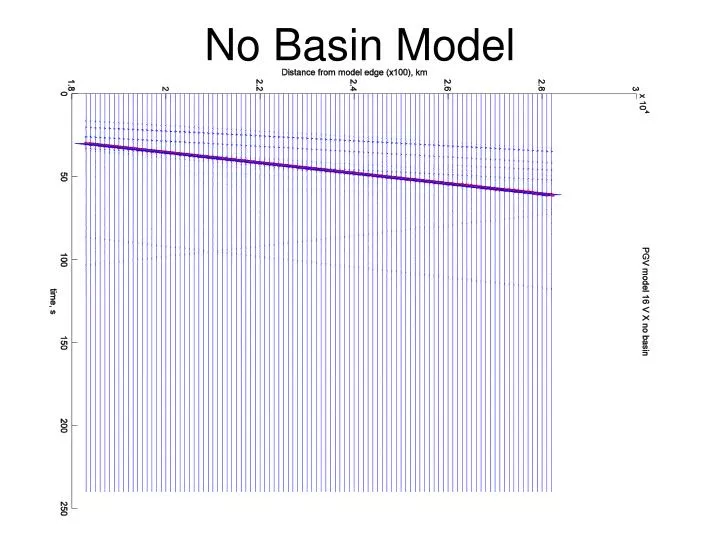
No Basin Model. Laterally Propagating Surface Wave Dominates. Near Surface Gradient. What do we see?. Laterally propagating surface wave dominated incoming energy. Deamplification caused by surface wave reflecting off basin edge due to high reflection coefficient.

E N D
Laterally Propagating Surface Wave Dominates
Near Surface Gradient
What do we see? • Laterally propagating surface wave dominated incoming energy. • Deamplification caused by surface wave reflecting off basin edge due to high reflection coefficient. • Phase loses coherency as wave propagates through basin • Frequency content still amplified.
Simple 2D One-Basin Model 2D models do show complex basin amplification in the frequency domain BUT • Cumulative RMS and PGV values show: • Higher vertical motion and energy. • Amplification and higher energy at basin edges. • Deamplification within and on the shadow side of the basin. Energy is unable to enter the basin structure. the basin appears to act as an energy screen.
Conclusions • The simplest 2D models are limited in their ability to portray basin response to seismic ground motion. 1D vertical complexity is not enough to produce results matching intuition. • Lateral complexity is required to produce expected basin amplification in ground motion e.g. intermediary basins, perhaps basin edge gradients. • Simple 2D models do produce spectral amplification. • This shows that expensive 3D model runs are one way to help characterize basin response, as 3D wave propagation allows more opportunity to put energy into the sides of basin features. • Inversion suggests the spatial pattern of ground motion depends strongly on incidence angle and type of incident waves. • Phase and incidence complexities influence basin amplification/deamplification. Also noted by Bravo and Sanchez-Sesma (1990).
AGU 2004 • Task: • Reproduce Hrvoje’s results to confirm deamplification seen in the UNR models is not due to bugs in codes.
Hrvoje’s model shows basin amplification in the time domain. • Verified that his sac outputs are reproducible at UNR. • Confirmed sac outputs in Aasha’s runs are identical to traces outputs. • Simple low velocity block shows amplification in the UNR velocity models. • confirmed deamplification seen in the UNR models is real and not dS\ue to code bugs
Simple 2D One-Basin Model 2D models do show complex basin amplification in the frequency domain BUT • Cumulative RMS and PGV values show: • Higher vertical motion and energy. • Amplification and higher energy at basin edges. • Deamplification within and on the shadow side of the basin. Energy is unable to enter the basin structure. the basin appears to act as an energy screen.
200 km 300 km 0 Hz 1 Hz
Statistical model to characterize Average Basin Response • Starting point: Misfit
Identify which variables reduce σ significantly • Four kinds of models
Next step will be: • source depth, D
Local basin depth and velocity contrasts are important. • The influence of Pg depth suggests that the mix of wave types propagating into the basin are an important factor on ground motion.
Reno Area Basin Response:Ground motion Simulation and basin response analyses A. Pancha, J. N. Louie, J. G. Anderson
Reno Area Basin • Our objective is to ascertain if 3D basin effects are significant. • The long-range goal is to achieve the ability to anticipate ground motion from future earthquakes in this rapidly growing urban area, with sufficient realism for engineering application.
Simulation of the Truckee 2/12/2002 Event • Magnitude Mw = 4.4 • Recorded on strong motion accelerometers within the Reno basin and on rock sites • Recorded on local network stations.
1D synthetic Green's functions, computed in a layered elastic solid using the generalized reflection and transmission coefficients (Luco and Apsel, 1983; Zeng & Anderson, 1995). • E3D • Compare these simulations with the real data
ID Parameters • Mo = 5.17E+22 dyne-cm Calculated: • Area = 0.894 km • Rise time = 0.69 seconds • Slip = 6.3 cm
E3D parameters • Grid spacing = 0.25 km • 77 by 99 km • Down to depth of 40 km • Rise time 0.7 seconds Gaussian STF • to = 0.5 seconds • Depth 11 km • dt = 0.015, t=4800 72 seconds
Truckee Event Mw = 4.4 13 km wide 21 km long
Results • 1. Good agreement is observed between the amplitudes of the synthetic 1D and 3D simulations • 2. 2D and 3D finite difference modeling matches the durations in the data and may anticipate some of the later arrivals. The 1D code does not. • 3. Ground motion amplitudes are greater within the basin than on the rock site. This is also reflected by the synthetic data, more so by the 3D results. • 4. A 3D model is required to simulate ground motion within the Reno area basin. • 5. Discrepancies between the amplitudes of the data and the synthetics suggest that either • - the community velocity model used to generate the synthetics presented here may contain basin sediments that are too stiff • - or the source strength of the Truckee event may be underestimated.