Download
1 / 46
460 likes | 581 Views
Klamath Basin Water Distribution Model Workshop. OUTLINE Brief Description of Water Distribution Models Model Setups Examples of networks and inputs Demand Estimates and Checks Two Simple Modeling Examples The Klamath Basin Question and Answers.

E N D
OUTLINE • Brief Description of Water Distribution Models • Model Setups • Examples of networks and inputs • Demand • Estimates and Checks • Two Simple Modeling Examples • The Klamath Basin • Question and Answers
Brief Description of Water Distribution Models What is a water distribution model? A water accounting system. Routes water within a distribution network (stream, canal, etc.) to demands based on priority and supply.
Basin Boundary Demands #1 and #2 normally would not compete for water because they are on different tributaries. However, due to the existence of a downstream demand (#3) with a senior priority date, there is an interaction between demands #1 and #2. Demand 1, 1967 priority Demand 2, 1905 priority Demand 3, 1865 priority Basin Outlet River
Model Setups • Network Examples and Data Requirements
Network Examples • General Network Description • The Ideal Network • The Workable Network • The Common Network
General Network Description • Links represent tributaries or streams • Source (inflow) nodes represent flows at • tributary confluence • Physical length of links are unimportant. Monthly time • step eliminates need to calculate travel times. • Relative placement of source nodes, demands and • tributary confluence are important.
General Network Description • Unknown • Parameters Physical Schematic Basin Boundary Source 1 Source 2 Source 3 Net Demand 1 Net Demand 2 Basin Outflow Tributary 2 Source 2 Source 1 Demand 1 Tributary 1 Demand 1 Tributary 3 • 3 Types Demand 2 Demand 2 Sources (Inflows) Net Demands Outflows Source 3 In aggregated terms, if any two parameters are known the third can be determine. Basin Outlet River Basin Outflow River
The Ideal Network • All demands, inflows and outflows within the basin • are measured. • No estimates required.
The Ideal Network Physical Schematic Flow Accounting Source 1 + Source 2 + Source 3 - Demand 1 - Demand 2 Gage Record Because of return flows, Sources -Demands Gage Flows Source 2 Basin Boundary Source 1 Demand 1 Demand 1 Demand 2 Demand 2 Source 3 Return flows can be directly calculated. Sources - Gage Record = Net Demands Demands -Net Demands = Return Flows River Gage River
The Workable Network. • Two out of three parameters are known. • inflows and outflows, or • inflows and demands, or • outflows and demands. • Other parameter can be calculated directly.
The Workable Network Physical Schematic Flow Accounting Source 2 Basin Boundary Source 1 Source 1 + Source 2 + Source 3 - Net Demand 1 - Net Demand 2 = Gage Record Calculated Net Demands directly (in aggregate terms) Demand 1 Demand 1 Source 3 Demand 2 Demand 2 Source Flows - Outflows = Net Demands Gage River River
Project Areas 1 and 2 are similar to the “workable network”. Net demands are calculated from gage records of inflows and outflows from the project.
The Common Network. • Only one out of three parameters are known. • (Usually sub-basin outflow). • Requires estimation of one of the unknown • parameters.
The Common Network Physical Schematic Flow Accounting Source 2 Basin Boundary Source 1 Source 1 + Source 2 + Source 3 - Net Demand 1 - Net Demand 2 = Gage Record Demand 1 Demand 1 Source 3 Demand 2 Need to estimate either source flows or net demands. Due to data limitations and time constraints, net demands were estimated in most areas above Klamath lake instead of source flows. Source flows can then be calculated according to the formula below. Demand 2 Gage Record + Net Demands = Source Flows (Zero Demand Flow) Gage River River
The Common Network Aggregated Physical Schematic Flow Accounting Source Flow Basin Boundary Gage Record + Net Demands = Source Flow OR Zero Demand Flow Demand 1 Net Demands Demand 2 This estimation of net demands and consequent calculation of source flows does not allow the modeling of the individual tributaries and demands. The demands and tributaries are aggregated. River Gage River
Network Example Summary • The Ideal Network - No estimates required Gage data • used directly to determine demands and flows. • The Workable Network - Net Demands are directly calculated. Demands may be Aggregated. • The Common Network - Estimates of either source flows • or net demands are required. Demands and source flows • are aggregated.
Demands • Estimates: How are net demands estimated? • Checks
Net Demand = (Evapotranspiration - Precipitation - Soil Moisture) x Acreage • Evapotranspiration estimated from Temperature • Records using Hargreaves Equation. • Precipitation taken from Rain Gage Data • Soil Moisture estimated using Soil Conservation Service Surveys, and Antecedent Precipitation • Crop Acreage
Example: Monthly Net Demand = (Evapotranspiration - Precipitation - Soil Moisture) x Acreage Monthly Net Demand = (7 inches - 0.5 inches - 0.5 inches) * 1000 acres = 500 ac-ft or 8.1 cfs
Demand Estimates Checks • Diversions • Simulated versus Measured • Canal Data • Depleted Flow Data • Annual Net Demand Estimates • Simulated versus Measured • Average • Yearly Trends • Annual Crop ET • Simulated versus “Agrimet” Data
Diversions • Simulated versus Measured Canal Data • Modoc Diversion Canal: • Comparison of simulated monthly average versus miscellaneous daily measurements.
Diversions • Simulated versus Measured Depleted Flows • Wood River 91-93: • Inflows from tributaries calculated from • miscellaneous records. • Demands estimated using previously described method. • Outflows taken from BOR gage data.
Physical Schematic Flow Accounting Source 2 Basin Boundary Source 1 Source 1 + Source 2 + Source 3 - Net Demand 1 - Net Demand 2 = Outflows Demand 1 Source 3 Demand 1 Demand 2 Demand 2 Compare Simulated Outflow to Gage data to check estimates Gage River
Diversion Check • Simulated diversions appear to be reasonable when compared to measured canal and depleted • flow data.
Annual Net Demand Estimates • Simulated average annual demand above Klamath Lake • versus measured average annual demand in the Project. • Climate is similar. • Same basin. • Demand is normalized by acreage (ac-ft/ac).
Annual Net Demand Estimates Check • Estimated annual demands above Klamath Lake appear reasonable when compared to measured data available elsewhere in the basin. • Yearly simulated variations in annual demands generally follow measured data.
Annual Crop ET • Simulated annual crop ET versus • “Agrimet” data in Lakeview.
Model Examples • Integrating Instream Demands • Single Tributary System • Two Tributary System
Actual Schematic Flow Accounting Basin Boundary Zero Demand Flows ZDF -Instream Demands = Flows Available for Irrigation Demands Demand 1 Demand 2 Demand A Instream Demands Instream Demand River River
Instream Demand C Counterintuitive Demand Interaction. ZDF Tributary A Instream demand D has a call on upstream demands. However, the shortages appear in Demand A instead of Demand B even through Demand A has a senior priority date. The reason is that instream demand C is effectively causing the shortages to Demand A, which consequently increases flows to instream demand D. Thus demand B is not called to reduce its use. Demand A, 1864 Demand B, 1905 ZDF Tributary B Instream Demand D
LEGEND Channels Source Nodes Consumptive Uses Junctions Marshes/Lakes GAUGE OVERLAP PERIOD (73-97) Accretions Middle Williamson ZDF Sycan ZDF Upper Williamson ZDF Lower Williamson Wood River and Tributaries ZDF Sprague Accretions Middle Sprague Other Tributaries Seeps and Springs Lake Ewauna Ewauna Accretions Project Area A1 LRDC Spencer Creek Project Area A2 Klamath Straits Drain