Download

1 / 51
510 likes | 706 Views
Evolution of Plasmodium falciparum var antigen genes. Przeworski lab meeting. Evolution of Plasmodium falciparum var genes. Malaria: a protozoan blood parasite carried by mosquito vectors principally of the genus Anopheles

E N D
Evolution of Plasmodium falciparum var antigen genes Przeworski lab meeting
Evolution of Plasmodium falciparum var genes • Malaria: a protozoan blood parasite carried by mosquito vectors principally of the genus Anopheles • Plasmodium falciparum and Plasmodium vivax are the main species infectious to humans • Related species infect primates, rodents, other mammals, birds and reptiles • P. falciparum is the most deadly: in humans it is responsible for • 80% of infections (250 million annually) • 90% of deaths (1 million annually) • Endemic in tropical and sub-tropical regions • Member of the Apicomplexa, a phylum characterized by a unique organelle called the apical complex/apicoplast responsible for lipid synthesis
Evolution of Plasmodium falciparum var genes • Key elements of life cycle: • Infection with diploid cells from mosquito bite • Asexual replication in liver and then red blood cells • Haploid cells produced in red blood cells, ingested by mosquito • Sex in mosquito produces diploid cells that migrate to saliavary gland • Cycles of replication and aggregation in blood vessels (sequestration) causes the symptoms of malaria: • Anaemia • Fever, chills, malaise • Coma (especially in cerebral malaria) • Sequestration prevents clearing of infected redblood cells by the spleen
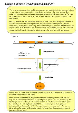
Evolution of Plasmodium falciparum var genes • The var genes are responsible for antigenic variation and sequestering by cytoadhesion • They encode PfEMP-1 (P. falciparum erythrocyte membrane protein), a parasite protein exported to the outside of the host red blood cells • Typically 60 var genes per genome, clustered telomerically. Differential expression allows immune evasion • Protein consists of Duffy binding-like domain (DBL) and cysteine-rich interdomain region (CIDR) • All proteins begin with DBL1, hence its use in population biology Kraemer et al. 2007 BMC Genomics 8:45
Evolution of Plasmodium falciparum var genes • Collaboration with Caroline Buckee (Oxford, Santa Fe and Kilifi) and Pete Bull (Kilifi) • Looking at 1000 DBL sequences • Aims • Investigate genetic structuring imposed by geography, selection and genomic position • Understand population biology: evidence for strain structure? • Reconstruct evolutionary history: quantify the roles of gene duplication, homologous and non-homologous recombination • Current hypotheses: • Categorization based on conserved 5’ regions and double-W • Recombination hierarchy • Some genotypes are over-represented in severe malaria
Evolution of Plasmodium falciparum var genes • Alignment is a major problem even in the conserved DBL domain • Multiple alignment algorithms • Clustal (Larkin et al. 2007 Bioinformatics 23: 2947-8) • Muscle (Edgar 2004 Nucleic Acids Research 32: 1792-7) • T-Coffee (Notredame et al. 2000 JMB 302: 205-17) • Pairwise alignment • BLAST (Tatiana et al. 1999 FEMS Microbiol Lett 174: 247-250) • Hidden Markov models (e.g. Lunter 2007 Bioinformatics 23: 2485-7) • Multiple statistical alignment • Phylogenetic (Holmes 2003 Bioinformatics S1: i147-57)
Malign: probabilistic sequence alignment in malariaas a pre-requisite for evolutionary inference • Simulating a sequence alignment • The likelihood of a sequence alignment • Bayesian inference • Testing, testing • Inference proper
Simulating an alignment: beta-binomial distribution • N=5 sequences, T=1 site • Simulate the frequency of indels from a symmetric beta distribution with parameters (,) • Given the frequency f, draw the number of indels from a binomial distribution with parameters (N,f)
Simulating an alignment: beta-binomial distribution • For example, the beta-binomial distribution with N=15 and • =0.1 (red) • =1 (yellow) • =10 (green) • The binomial distribution with p=0.5 (blue)
Simulating nucleotides: multinomial-Dirichlet distribution • Simulate the nucleotide frequencies from a symmetric Dirichlet distribution with parameter =(,,,) • Given the frequencies f=(fA, fG, fC, fT), simulate the number of As Gs Cs and Ts from a multinomial distribution with parameters (N,f) = 0.1 = 1 = 10
Simulating a nucleotide alignment T = 100 L = 77
Simulating a nucleotide alignment True alignment Raw data
Representing an alignment • Matrix of size N by L • 0 indicates an indel • Other integers correspond to the position in the raw sequence
The likelihood of an alignment: indel pattern • Let I be the number of indels, and be the parameter of the beta distribution. N is the number of sequences. • For a single column in the alignment, the beta-binomial distribution gives the probability of I • However, the sequences are labelled, so the ordering matters. Therefore the likelihood is
The likelihood of an alignment: nucleotide pattern • Let Yi, i={A,G,C,T} be the number of each type of nucleotide in the remaining (N-I) non-indels. Let be the parameter of the Dirichlet distribution. • For a single column, conditional on the indel pattern, the multinomial-Dirichlet distribution gives the likelihood of Y • Again the ordering matters, so the likelihood is
The likelihood of an alignment: missing columns • Because our representation of the alignment does not specify the exact position of columns fixed for indels, we need to take that into account in the likelihood. • When there are (T-L) columns fixed for indels, their likelihood is
Review of assumptions • Independence between sites = free recombination • Exchangeability between sequences = panmictic population structure • Equal base usage and stationary frequency distribution • Simplistic indel model
Bayesian inference • Fix the auxiliary variables, e.g. at N=15 and T=100 • Priors on and , e.g. exponential distribution with mean 0.1 • Markov chain Monte Carlo (MCMC) for sampling from the joint posterior distribution of , and the alignment
MCMC: Multiplicative updates to and • E.g. propose an update from to ´: • Let U ~ Uniform(-1,1) • Let ´ = exp(U) • The acceptanceprobability is
MCMC: Updating the alignment • General strategy is to partition the current alignment at random
MCMC: Updating the alignment • And re-align one partition relative to the other
MCMC: Updating the alignment • Gaps are stripped from both
MCMC: Updating the alignment 0 1 2 3 4 5 6 7 8 9 10 11 12 13 14 15 16 17 18 19 20 21 22 • And the reference partition (top) is labelled • Odd-numbered sites correspond to gaps, even-numbered sites to matches
MCMC: Updating the alignment 0 1 2 3 4 5 6 7 8 9 10 11 12 13 14 15 16 17 18 19 20 21 22 • Each site in the non-reference partition is aligned to a numbered site in the reference partition
MCMC: Updating the alignment 0 1 2 3 4 5 6 7 8 9 10 11 12 13 14 15 16 17 18 19 20 21 22 • Gaps may have multiple hits, but matches cannot 0 0 1 7 11 15 17 18 21
MCMC: Updating the alignment • Finally the alignment is reconstructed
MCMC: Updating the alignment • In this example, it has grown by two columns
0 1 2 3 4 5 6 7 8 9 10 11 12 13 14 15 16 17 18 19 20 21 22 0 0 1 7 11 15 17 18 21 MCMC: Updating the alignment Partitioning the alignment probabilistic Stripping indels book-keeping Realigning the partitions probabilistic Reconstructing the alignment book-keeping
MCMC: Partitioning the alignment • The partition size is drawn from some discrete distribution between 1 and N-1, e.g. uniform, or inverse. • Sequences are then assigned to one partition or the other uniformly at random (formally, the hypergeometric distribution describes this method of sampling without replacement). • The proposal probability is independent of the alignment, so the ratio of reverse and forward proposal probabilities (the Hastings ratio) is 1.
0 1 2 3 4 5 6 7 8 9 10 11 12 13 14 15 16 17 18 19 20 21 22 0 0 1 7 11 15 17 18 21 MCMC: Realigning the partitions • In principal, you could enumerate over all possible alignments of the non-reference to the reference partition. (Very approximately (2L)L combinations). • For each combination you could calculate the posterior probability and Gibbs sample. • In practice, not computationally tractable so I impose a window of, e.g. ±40 matches, which constrains the maximum distance a site in the non-reference partition can move from its current position. • The likelihood can be calculated it an efficient manner (computer scientists would call it dynamic programming).
0 1 2 3 4 5 6 7 8 9 10 11 12 13 14 15 16 17 18 19 20 21 22 0 0 1 7 11 15 17 18 21 MCMC: Realigning the partitions • Since not all possible moves are allowed, the proposal is a Metropolis-Hastings move. • To calculate the reverse proposal probability for the Hastings ratio, it is necessary to implement the move and carry out the full computations a second time. • The proposed change in the alignment, A´, is accepted with the usual probability
R/C implementation • The MCMC code is written in C for speed • Linked as a static library and called from R for graphical monitoring and post-processing • Can watch the chain and the current alignment in real time
Testing, testing • It is criminally insane to assume your MCMC will work (straight away) • Two methods of testing are highly recommended • Do you retrieve the prior when there is no data? • Is the posterior well-calibrated?
Do you retrieve the prior when there is no data? • Testing the prior for alpha and beta is straightforward: you feed the program no data and compare to the specified prior distribution. • How do you test the “prior” on the alignment? • The “prior” on the alignment is conditional on the sequence lengths but not on the nucleotide sequences themselves • Calculate it theoretically for sufficiently simple examples • Use an alternative method for sampling from the prior, such as importance sampling, and compare.
Testing the alignment prior: theoretical approach • For the 2-sequence case, this is theoretically tractable. Suppose both sequences have length S, and the maximum alignment length is T. Calculate the alignment length Pr(L|S). Configuration Count Prior probability 2S-L L-S L-S T-L
Testing the alignment prior: theoretical approach • E.g.T=100, S=50, =0.1 • Key • MCMC: black lines • Theory: red lines
Testing the alignment prior: importance sampling • Importance sampling is an alternative to MCMC. • Instead of proposing local moves to the parameters and missing data, they are independently proposed de novo each iteration. • Each simulation is given a weighting equal to the ratio of the posterior and proposal probabilities. • The proposal distribution is chosen to approximate the posterior distribution, and thus minimize the variance in the weightings. • I used a sequential importance sampler (SIS) that simulates the first sequence, then the second given the first, and so on. • Each sequence is simulated to ensure agreement with the observed sequence length. • The importance sampler represents a better choice for simulating from the prior, but not necessarily the posterior.
Testing the alignment prior: importance sampling • E.g.N=15, T=100, =0.3S=[51, 52, 47, 47, 57, 47, 50, 53, 48, 49, 44, 47, 52, 50, 50] • Key • MCMC: white bars 3000 iterations • SIS: grey bars 1000 iterations
Is the posterior well-calibrated? • The well-calibrated Bayesian is a person whose prior beliefs reflect the long-run probabilities of an event. • Dawid, A.P. (1982) JASA 77: 605-10 • For example, if a weather forecaster predicts the chance of rain each day, s/he is well calibrated if, in the long-run, it rained on at least 80% of the days when the predicted chance of rain was 80% or more. • This is a minimum requirement for good inference: a lazy weather forecaster would be well-calibrated if s/he used the annual precipitation rate as his/her estimated chance of rain every day.
Is the posterior well-calibrated? • The idea of calibration can be used to test a Bayesian inference procedure, using the following simulation scheme • Simulate a parameter from a prior p() • Simulate data X from a model p(X|) • Perform inference using the same prior and likelihood to obtain a posterior distribution phat(|X) • Calculate a 95% credible interval based on phat(|X) • Repeat many times • If the method of inference is working correctly, the credible intervals must be well-calibrated. • A calibration curve shows the proportion of simulations for which the true value of fell within the 100(1-)% credible interval. • To be well-calibrated means that proportion equals 1-
Debugging • Check the likelihood calculations are consistent • For accepted moves, check the calculated reverse move probability was correct • Go through the calculations for simple examples by hand • Theory - go through again by hand
Inference proper • Screw debugging, let’s analyse the data • What will we do with a posterior distribution of sequence alignments? • For inference • Improper inverse priors on and • Improper uniform distribution on the maximum alignment length T