Download
1 / 24
241 likes | 783 Views
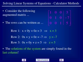
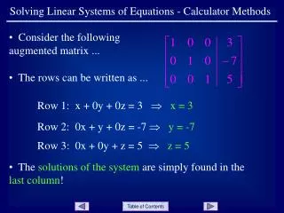
Solving Linear Systems: Iterative Methods and Sparse Systems. COS 323. Direct vs. Iterative Methods. So far, have looked at direct methods for solving linear systems Predictable number of steps No answer until the very end Alternative: iterative methods Start with approximate answer

E N D
Solving Linear Systems:Iterative Methods and Sparse Systems COS 323
Direct vs. Iterative Methods • So far, have looked at direct methods forsolving linear systems • Predictable number of steps • No answer until the very end • Alternative: iterative methods • Start with approximate answer • Each iteration improves accuracy • Stop once estimated error below tolerance
Benefits of Iterative Algorithms • Some iterative algorithms designed for accuracy: • Direct methods subject to roundoff error • Iterate to reduce error to O() • Some algorithms produce answer faster • Most important class: sparse matrix solvers • Speed depends on # of nonzero elements,not total # of elements • Today: iterative improvement of accuracy,solving sparse systems (not necessarily iteratively)
Iterative Improvement • Suppose you’ve solved (or think you’ve solved) some system Ax=b • Can check answer by computing residual: r = b – Axcomputed • If r is small (compared to b), x is accurate • What if it’s not?
Iterative Improvement • Large residual caused by error in x: e = xcorrect – xcomputed • If we knew the error, could try to improve x: xcorrect = xcomputed + e • Solve for error: Axcomputed = A(xcorrect – e) = b – r Axcorrect – Ae = b – r Ae = r
Iterative Improvement • So, compute residual, solve for e,and apply correction to estimate of x • If original system solved using LU,this is relatively fast (relative to O(n3), that is): • O(n2) matrix/vector multiplication +O(n) vector subtraction to solve for r • O(n2) forward/backsubstitution to solve for e • O(n) vector addition to correct estimate of x
Sparse Systems • Many applications require solution oflarge linear systems (n = thousands to millions) • Local constraints or interactions: most entries are 0 • Wasteful to store all n2 entries • Difficult or impossible to use O(n3) algorithms • Goal: solve system with: • Storage proportional to # of nonzero elements • Running time << n3
Special Case: Band Diagonal • Last time: tridiagonal (or band diagonal) systems • Storage O(n): only relevant diagonals • Time O(n): Gauss-Jordan with bookkeeping
Cyclic Tridiagonal • Interesting extension: cyclic tridiagonal • Could derive yet another special case algorithm,but there’s a better way
Updating Inverse • Suppose we have some fast way of finding A-1for some matrix A • Now A changes in a special way: A* = A + uvTfor some n1 vectors u and v • Goal: find a fast way of computing (A*)-1 • Eventually, a fast way of solving (A*)x = b
Applying Sherman-Morrison • Let’s considercyclic tridiagonal again: • Take
Applying Sherman-Morrison • Solve Ay=b, Az=u using special fast algorithm • Applying Sherman-Morrison takesa couple of dot products • Total: O(n) time • Generalization for several corrections: Woodbury
More General Sparse Matrices • More generally, we can represent sparse matrices by noting which elements are nonzero • Critical for Ax and ATx to be efficient:proportional to # of nonzero elements • We’ll see an algorithm for solving Ax=busing only these two operations!
Compressed Sparse Row Format • Three arrays • Values: actual numbers in the matrix • Cols: column of corresponding entry in values • Rows: index of first entry in each row • Example: (zero-based) values 3 2 3 2 5 1 2 3 cols 1 2 3 0 3 1 2 3 rows 0 3 5 5 8
Compressed Sparse Row Format • Multiplying Ax:for (i = 0; i < n; i++) { out[i] = 0; for (j = rows[i]; j < rows[i+1]; j++) out[i] += values[j] * x[ cols[j] ];} values 3 2 3 2 5 1 2 3 cols 1 2 3 0 3 1 2 3 rows 0 3 5 5 8
Solving Sparse Systems • Transform problem to a function minimization! Solve Ax=b Minimize f(x) = xTAx – 2bTx • To motivate this, consider 1D: f(x) = ax2 – 2bxdf/dx = 2ax – 2b = 0 ax = b
Solving Sparse Systems • Preferred method: conjugate gradients • Recall: plain gradient descent has a problem…
Solving Sparse Systems • … that’s solved by conjugate gradients • Walk along direction • Polak and Ribiere formula:
Solving Sparse Systems • Easiest to think about A = symmetric • First ingredient: need to evaluate gradient • As advertised, this only involves A multipliedby a vector
Solving Sparse Systems • Second ingredient: given point xi, direction di,minimize function in that direction
Solving Sparse Systems • So, each iteration just requires a fewsparse matrix – vector multiplies(plus some dot products, etc.) • If matrix is nn and has m nonzero entries,each iteration is O(max(m,n)) • Conjugate gradients may need n iterations for“perfect” convergence, but often get decent answer well before then