Download
1 / 16
250 likes | 633 Views
Direct Methods Systematic transformation of system of equations into equivalent systems, until the unknown variables are easily solved for. Iterative methods

E N D
Direct Methods Systematic transformation of system of equations into equivalent systems, until the unknown variables are easily solved for. Iterative methods Starting with an initial “guess” for the unknown vector, successively “improve” the guess, until it is “sufficiently” close to the solution. Solution of Sparse Linear Systems
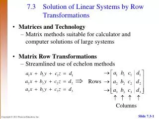
Direct Solution of Linear SystemsGaussian Elimination div by 2 *(-1) *(-3) • Unknowns solved by back-substitution after Gaussian Elimination
More efficient than Gaussian Eimination when solving many systems with the same coefficient matrix. First A is decomposed into product: A = LU To solve linear system Ax=b, we need to solve (LU)x=b Let z=Ux; we have L(Ux)=b, or Lz=b. This can be solved for z by forward-substitution. Since Ux=z, and z is now known, we can solve for x by back-substitution. LU Decomposition =
If A is symmetric and positive definite , it can be factored in the form Cholesky factorization requires only around half as many arithmetic operations as LU decomposition. The forward and back-substitution process is the same as with LU decomposition. Cholesky Factorization =
A significant fraction of matrix elements are known to be zero, e.g. matrix arising from a finite-difference discretization of a PDE: At most 5 non-zero elements in any row of the matrix, irrespective of the size of the matrix (number of grid points). Sparse matrix is represented in some compact form that keeps information about the non-zero elements. 1 2 3 4 5 6 Sparse Linear Systems 1 2 3 4 5 6 1 4 -1 0 -1 0 0 2 -1 4 -1 0 -1 0 3 0 -1 4 0 -1 -1 4 -1 0 0 4 -1 0 5 0 -1 0 -1 4 -1 6 0 0 -1 0 -1 4
For a 100 by 100 grid, with a finite difference discretization using a 5-point stencil, less than .05% of the matrix elements are non-zero. 2 2 2 2 2 n n n n n Resulting sparse matrix x Sparse Linear Systems 1 1 n Physical nxn Grid
A commonly used representation for sparse matrices: Compressed Sparse Row Format 0 1 2 3 4 5 0 4 -1 0 -1 0 0 1 -1 4 -1 0 -1 0 2 0 -1 4 0 0 -1 3 -1 0 0 4 -1 0 4 0 -1 0 -1 4 -1 5 0 0 -1 0 -1 4 rb 0 3 7 10 13 17 20 a 4 -1 -1 -1 4 -1 -1 -1 4 -1 -1 4 -1 -1 -1 4 -1 -1 -1 4 0 1 2 3 4 5 6 7 8 9 10 11 12 13 14 15 16 17 18 19 0 1 3 0 1 2 4 1 2 5 0 3 4 1 3 4 5 2 4 5 col for (i = 0; i<n; i++) for(j=rb[i];j<rb[i+1];j++) y[i] += a[j]*x[col[j]]; Sparse MV Multiply for (i = 0; i<n; i++) for(j=0;j<n;j++) y[i] += a[i][j]*x[j]; Dense MV Multiply
During solution of sparse linear system (by GE or LU or Cholesky), row-updates often result in creation of non-zero entries that were originally zero. Row updates using row-1 result in fill-in non-zeros (F). Fill-in Non-Zeros
Re-ordering the equations (rows) or unknowns (columns) can result in significant change in the number of fill-in non-zeros, and hence time for matrix factorization. Effect of reordering on fill-in Fill-in with GE Reorder rows/cols No fill-in with GE
A graph-based view of matrix’s sparsity structure is extremely useful in generating low-fill re-orderings. The associated graph of a symmetric sparse matrix has a vertex corresponding to each row/col. of matrix, and an edge corresponding to each non-zero matrix entry. 4 1 2 3 6 5 Associated graph of matrix
Row-i updates row-j, j>i iff Aji is non-zero; in the associated graph a matrix non-zero corresponds to an edge. Row-update(i->j) could cause fill-in non-zero Ajk corresponding to all non-zeros Aik. After all updates from row-i, all neighbors of vertex i in the associated graph form a clique. Fill-in and graph transformation l l i i j j k k
Each row’s effect on fill-in generation is captured by the “clique” transformation on the associated graph. The graph view is valuable in suggesting matrix re-ordering approaches. 4 1 2 3 4 4 5 6 1 1 2 2 3 3 5 5 6 6 Fill-in and graph transformation 4 1 2 3 5 6
Graph-based algorithm for generating low-fill re-ordering. Matrix permutation is viewed as node-numbering problem in associated graph. Low-degree nodes are numbered early - so that they are removed without adding many fill-in edges. For example, minimum-degree finds a no-fill ordering. d=1 1 1 1 1 d=2 d=2 d=2 d=3 4 d=3 d=3 d=2 d=1 d=3 d=3 d=2 d=2 d=1 d=3 d=1 d=1 2 d=1 2 3 2 3 d=1 d=1 Matrix re-ordering: Minimum Degree
4 1 2 3 6 5 Re-ordered matrix 1 4 5 6 3 2
Find a minimal vertex-separator to bisect associated graph; number those nodes last; recursively apply to both halves. Property: Given a numbering of nodes, fill-in Aij exists, j>i, iff there is a path from i to j in graph using only lower numbered vertices. No fill-in edges between one half and other half of partition. 1-21 19 21 43 49 40 42 22-42 Matrix re-ordering: Nested Dissection
Comparison of Ordering Schemes Number of non-zeros after fill-in Sparse matrix factorization time