Download
1 / 9
90 likes | 217 Views
Sparse Systems and Iterative Methods. Paul Heckbert Computer Science Department Carnegie Mellon University. PDE’s and Sparse Systems. A system of equations is sparse when there are few nonzero coefficients, e.g. O( n ) nonzeros in an n x n matrix.

E N D
Sparse Systems and Iterative Methods Paul Heckbert Computer Science Department Carnegie Mellon University 15-859B - Introduction to Scientific Computing
PDE’s and Sparse Systems • A system of equations is sparse when there are few nonzero coefficients, e.g. O(n) nonzeros in an nxn matrix. • Partial Differential Equations generally yield sparse systems of equations. • Integral Equations generally yield dense (non-sparse) systems of equations. • Sparse systems come from other sources besides PDE’s. 15-859B - Introduction to Scientific Computing
Example: PDE Yielding Sparse System • Laplace’s Equation in 2-D: 2u = uxx +uyy = 0 • domain is unit square [0,1]2 • value of function u(x,y) specified on boundary • solve for u(x,y) in interior 15-859B - Introduction to Scientific Computing
Sparse Matrix Storage • Brute force: store nxn array, O(n2) memory • but most of that is zeros – wasted space (and time)! • Better: use data structure that stores only the nonzeros col 1 2 3 4 5 6 7 8 9 10... val 0 1 0 0 1 -4 1 0 0 1... 16 bit integer indices: 2, 5, 6, 7,10 32 bit floats: 1, 1,-4, 1, 1 • Memory requirements, if kn nonzeros: • brute force: 4n2 bytes, sparse data struc: 6kn bytes 15-859B - Introduction to Scientific Computing
An Iterative Method: Gauss-Seidel • System of equations Ax=b • Solve ith equation for xi: • Pseudocode: until x stops changing for i = 1 to n x[i] (b[i]-sum{ji}{a[i,j]*x[j]})/a[i,i] • modified x values are fed back in immediately • converges if A is symmetric positive definite 15-859B - Introduction to Scientific Computing
Variations on Gauss-Seidel • Jacobi’s Method: • Like Gauss-Seidel except two copies of x vector are kept, “old” and “new” • No feedback until a sweep through n rows is complete • Half as fast as Gauss-Seidel, stricter convergence requirements • Successive Overrelaxation (SOR) • extrapolate between old x vector and new Gauss-Seidel x vector, typically by a factor between 1 and 2. • Faster than Gauss-Seidel. 15-859B - Introduction to Scientific Computing
Conjugate Gradient Method • Generally for symmetric positive definite, only. • Convert linear system Ax=b • into optimization problem: minimize xTAx-xTb • a parabolic bowl • Like gradient descent • but search in conjugate directions • not in gradient direction, to avoid zigzag problem • Big help when bowl is elongated (cond(A) large) 15-859B - Introduction to Scientific Computing
Conjugate Directions 15-859B - Introduction to Scientific Computing
Convergence ofConjugate Gradient Method • If K = cond(A) = max(A)/ min(A) • then conjugate gradient method converges linearly with coefficient (sqrt(K)-1)/(sqrt(K)+1) worst case. • often does much better: without roundoff error, if A has m distinct eigenvalues, converges in m iterations! 15-859B - Introduction to Scientific Computing