Download
1 / 125
1.26k likes | 1.57k Views
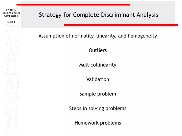
Strategy for Complete Discriminant Analysis. Assumption of normality, linearity, and homogeneity Outliers Multicollinearity Validation Sample problem Steps in solving problems Homework problems. Assumptions of normality, linearity, and homogeneity of variance.

E N D
Strategy for Complete Discriminant Analysis Assumption of normality, linearity, and homogeneity Outliers Multicollinearity Validation Sample problem Steps in solving problems Homework problems
Assumptions of normality, linearity, and homogeneity of variance • The ability of discriminant analysis to extract discriminant functions that are capable of producing accurate classifications is enhanced when the assumptions of normality, linearity, and homogeneity of variance are satisfied. • We will use the script for testing for normality and test substituting the log, square root, or inverse transformation when they induce normality in a variable that fails to satisfy the criteria for normality. • We can compare the accuracy rates in a model using transformed variables to one that does not to evaluate whether or not the improvement gained by transformed variables is sufficient to justify the interpretational burden of explaining transformations.
Assumption of linearity in discriminant analysis • Since the dependent variable is non-metric in discriminant analysis, there is not a linear relationship between the dependent variable and an independent variable. • In discriminant analysis, the assumption of linearity applies to the relationships between pairs of independent variable. To identify violations of linearity, each metric independent variable would have to be tested against all others. • Since non-linearity only reduces the power to detect relationships, the general advice is to attend to it only when we know that a variable in our analysis consistently demonstrated non-linear relationships with other independent variables. • We will not test for linearity in our problems.
Assumption of homogeneity of variance - 1 • The assumption of homogeneity of variance is particular important in the classification stage of discriminant analysis. • If one of the groups defined by the dependent variable has greater dispersion than others, cases will tend to be over classified in it. • Homogeneity of variance is tested with Box's M test, which tests the null hypotheses that the group variance-covariance matrices are equal. If we fail to reject this null hypothesis and conclude that the variances are equal, we use the SPSS default of using a pooled covariance matrix in classification. • If we reject the null hypothesis and conclude that the variances are heterogeneous, we substitute separate covariance matrices in the classification, and evaluate whether or not our classification accuracy is improved.
Assumption of homogeneity of variance - 2 SPSS does not calculate a cross-validated accuracy rate when it uses separate covariance matrices in classification. When we use separate covariance matrices in classification, the decision to use the baseline or the revised model is based on the accuracy rates that SPSS identifies as the % of original grouped cases correctly classified.
Detecting outliers in discriminant analysis - 1 • In the classification phase of discriminant analysis, each case will be predicted to be a member of one of the groups defined by the dependent variable. • The assignment is based on proximity, i.e. the case will be assigned to the group it is closest to in multidimensional space. • Just as we use z-scores to measure the location of a case in a distribution with a given mean and standard deviation, we can use Mahalanobis distance as a measure of the location of a case relative to the centroid and covariance matrix for the cases in the distribution for a group of cases. The centroid and covariance matrix are the multivariate equivalents of a mean and standard deviation.
Detecting outliers in discriminant analysis - 2 • According to the SPSS Base 10.0 Applications Guide, page 259, "cases with large values of Mahalanobis distance from their group mean can be identified as outliers." • In the Casewise Statistics output, SPSS provides us with the Squared Mahalanobis Distance to the Centroid for each of the groups defined by the dependent variable. • If a case has a large Squared Mahalanobis Distance to the Centroid is most likely to belong to, it is an outlier.
Detecting outliers in discriminant analysis - 3 • If we calculate the critical value that identifies a "large" value for Mahalanobis D² distance, we can scan the Casewise Statistics table to identify outliers. • When we identified multivariate outliers, we used the SPSS function CDF.CHISQ to calculate the probability of obtaining a D² of a certain size, given the number of independent variables in the analysis. • SPSS has a parallel function, IDF.CHISQ, that computes the size of D² needed to reach a specific probability, given the number of independent variables in the analysis.
Detecting outliers in discriminant analysis - 4 • Since we are dealing with the classification phase of discriminant analysis, we use the number of independent variables included in computing the discriminant scores for cases. • For simultaneous discriminant analysis in which all independent variables are entered at the same time, we use the total number of independent variables in the calculations for the critical value for D². • For stepwise discriminant analysis, in which variables are entered by statistical criteria, we use the number of variables satisfying the statistical criteria in the calculations for the critical value for D².
Detecting outliers in discriminant analysis - 5 • We will identify outliers as cases whose probability of being in the group that they are most likely to belong it is 0.01 or less. Since the IDF.CHISQ function is based on cumulative probabilities from the left tail of the distribution through the critical value, we will use 1.00 – 0.01 = 0.99 as the probability in the IDF.CHIDQ function. • For simultaneous discriminant analysis with 4 independent variables, the compute command for the critical value of D² is: COMPUTE critval = IDF.CHISQ(0.99, 4). • For stepwise discriminant analysis, in which 2 of for independent variables, the compute command for the critical value of D² is: COMPUTE critval = IDF.CHISQ(0.99, 2).
Multicollinearity • Multicollinearity has the same effect in discriminant analysis that it does in multiple regression, i.e. the importance of an independent variable will be undervalued because it has a very strong relationship to another independent variable or combination of independent variables. • Like multiple regression, multicollinearity in discriminant analysis is identified by examining tolerance values. • While tolerance is routinely included in the output for the stepwise method for including variables, it is not included for simultaneous entry of variables. If a tolerance problem occurs in a simultaneous entry problem, SPSS will include a table titled "Variables Failing Tolerance Test." • We should not attempt to interpret an analysis with a multicollinearity problem until we have resolved the problem by removing or combining the problematic variable.
Validation • The primary criteria for a successful discriminant analysis are: • the existence of sufficient statistically significant discriminant functions to distinguish among the groups defined by the dependent variable, and • an accuracy rate that substantially improves the accuracy rate obtainable by chance alone. • SPSS calculates a cross-validated accuracy rate for the analysis, using a jackknife or leave-one-out at a time strategy. It computes the discriminant analysis once for each case in the sample, leaving the case out of the calculations for the discriminant model. The discriminant model is then used to classify the case that was left out or held out. Thus the bias toward an optimistically high accuracy rate is avoided. • We will use this cross-validation in our problems rather than doing a separate 75-25% cross-validation.
Overall strategy for solving problems • Run a baseline discriminant analysis using the method for including variables implied by the problem statement to find the baseline cross-validated accuracy rate for the model. • Test for useful transformations to improve normality. • Substitute transformed variables and check for outliers. • If cross-validated accuracy rate from discriminant analysis using transformed variables and omitting outliers is at least 2% better than baseline cross-validated accuracy rate, select it for interpretation; otherwise select baseline model. • If the Box’s M statistic is statistically significant, we violate the assumption of homogeneity of variance and re-run the analysis using separate covariance matrices for classification. If the accuracy rate increases by more than 2%, we interpret this model, otherwise return to model using pooled covariance. • If the cross-validated accuracy rate is 25% or more higher than proportional by chance accuracy rate, interpret the selected discriminant model: • Number of functions and importance of predictors • Role of individual variables on functions distinguishing among groups
Discriminant analysis – stepwise variable entry The first question requires us to examine the level of measurement requirements for discriminant analysis. Standard discriminant analysis requires that the dependent variable be nonmetric and the independent variables be metric or dichotomous.
Level of measurement - answer Standard discriminant analysis requires that the dependent variable be nonmetric and the independent variables be metric or dichotomous. True with caution is the correct answer.
Sample size requirements The second question asks about the sample size requirements for discriminant analysis. To answer this question, we will run the discriminant analysis to obtain some basic data about the problem and solution. The phrase “best subset of predictors” is our clue that we should use the stepwise method for including variables in the model.
The stepwise discriminant analysis – baseline model To answer the question, we do a stepwise discriminant analysis with natfare as the dependent variable and hrs1, wkrslf, educ, and rincom98, and as the independent variables. Select the Classify | Discriminant… command from the Analyze menu.
Selecting the dependent variable First, highlight the dependent variable natfare in the list of variables. Second, click on the right arrow button to move the dependent variable to the Grouping Variable text box.
Defining the group values When SPSS moves the dependent variable to the Grouping Variable textbox, it puts two question marks in parentheses after the variable name. This is a reminder that we have to enter the number that represent the groups we want to include in the analysis. First, to specify the group numbers, click on the Define Range… button.
Completing the range of group values • The value labels for natfare show three categories: • 1 = TOO LITTLE • 2 = ABOUT RIGHT • 3 = TOO MUCH • The range of values that we need to enter goes from 1 as the minimum and 3 as the maximum. First, type in 1 in the Minimum text box. Second, type in 3 in the Maximum text box. Third, click on the Continue button to close the dialog box. Note: if we enter the wrong range of group numbers, e.g., 1 to 2 instead of 1 to 3, SPSS will only include groups 1 and 2 in the analysis.
Specifying the method for including variables SPSS provides us with two methods for including variables: to enter all of the independent variables at one time, and a stepwise method for selecting variables using a statistical test to determine the order in which variables are included. Since the problem calls for identifying the best predictors, we click on the option button to Use stepwise method.
Requesting statistics for the output Click on the Statistics… button to select statistics we will need for the analysis.
Specifying statistical output First, mark the Means checkbox on the Descriptives panel. We will use the group means in our interpretation. Second, mark the Univariate ANOVAs checkbox on the Descriptives panel. Perusing these tests suggests which variables might be useful descriminators. Third, mark the Box’s M checkbox. Box’s M statistic evaluates conformity to the assumption of homogeneity of group variances. Fourth, click on the Continue button to close the dialog box.
Specifying details for the stepwise method Click on the Method… button to specify the specific statistical criteria to use for including variables.
Details for the stepwise method First, mark the Mahalanobis distance option button on the Method panel. Second, mark the Summary of steps checkbox to produce a summary table when a new variable is added. Third, click on the Continue button to close the dialog box. Fourth, type the level of significance in the Entry text box. The Removal value is twice as large as the entry value. Third, click on the option button Use probability of F so that we can incorporate the level of significance specified in the problem.
Specifying details for classification Click on the Classify… button to specify details for the classification phase of the analysis.
Details for classification - 1 First, mark the option button to Compute from group sizes on the Prior Probabilities panel. This incorporates the size of the groups defined by the dependent variable into the classification of cases using the discriminant functions. Second, mark the Casewise results checkbox on the Display panel to include classification details for each case in the output. Third, mark the Summary table checkbox to include summary tables comparing actual and predicted classification.
Details for classification - 2 Fourth, mark the Leave-one-out classification checkbox to request SPSS to include a cross-validated classification in the output. This option produces a less biased estimate of classification accuracy by sequentially holding each case out of the calculations for the discriminant functions, and using the derived functions to classify the case held out.
Details for classification - 3 Fifth, accept the default of Within-groups option button on the Use Covariance Matrix panel. The Covariance matrices are the measure of the dispersion in the groups defined by the dependent variable. If we fail the homogeneity of group variances test (Box’s M), our option is use Separate groups covariance in classification. Seventh, click on the Continue button to close the dialog box. Sixth, mark the Combined-groups checkbox on the Plots panel to obtain a visual plot of the relationship between functions and groups defined by the dependent variable.
Completing the discriminant analysis request Click on the OK button to request the output for the discriminant analysis.
Sample size – ratio of cases to variablesevidence and answer The minimum ratio of valid cases to independent variables for discriminant analysis is 5 to 1, with a preferred ratio of 20 to 1. In this analysis, there are 138 valid cases and 4 independent variables. The ratio of cases to independent variables is 34.5 to 1, which satisfies the minimum requirement. In addition, the ratio of 34.5 to 1 satisfies the preferred ratio of 20 to 1.
Sample size – minimum group sizeevidence and answer In addition to the requirement for the ratio of cases to independent variables, discriminant analysis requires that there be a minimum number of cases in the smallest group defined by the dependent variable. The number of cases in the smallest group must be larger than the number of independent variables, and preferably contain 20 or more cases. The number of cases in the smallest group in this problem is 32, which is larger than the number of independent variables (4), satisfying the minimum requirement. In addition, the number of cases in the smallest group satisfies the preferred minimum of 20 cases. In this problem we satisfy both the minimum and preferred requirements for ratio of cases to independent variables and minimum group size. For this problem, true is the correct answer.
Classification accuracy before transformations or removing outliers Prior to any transformations of variables to satisfy the assumptions of discriminant analysis or removal of outliers, the cross-validated accuracy rate was 50.0%. This accuracy rate is the benchmark that we will use to evaluate the utility of transformations and the elimination of outliers.
Assumption of normality of independent variable - question Having satisfied the level of measurement and sample size requirements, we turn our attention to conformity with the assumption of normality, the detection of outliers, and the assumption of homogeneity of the covariance matrices used in classification. First, we will evaluate the assumption of normality for the first independent variable.
Test Assumption of Normality with Script First, move the variables to the list boxes based on the role that the variable plays in the analysis and its level of measurement. Second, click on the Assumption ofNormality option button to request that SPSS produce the output needed to evaluate the assumption of normality. Fourth, mark the dependent variable as nonmetric. Third, mark the checkboxes for the transformations that we want to test in evaluating the assumption. Fifth, click on the OK button to produce the output.
Assumption of normality of independent variable – evidence and answer The variable "number of hours worked in the past week" [hrs1] satisfies the criteria for a normal distribution. The skewness (-0.324) and kurtosis (0.935) were both between -1.0 and +1.0. The answer to the question is true.
Assumption of normality of independent variable - question Next, we will evaluate the assumption of normality for the second independent variable.
Assumption of normality of independent variable – evidence and answer The independent variable "highest year of school completed" [educ] does not satisfy the criteria for a normal distribution. The skewness (-0.137) fell between -1.0 and +1.0, but the kurtosis (1.246) fell outside the range from -1.0 to +1.0.
Assumption of normality of independent variable – evidence and answer Neither the logarithmic, the square root, nor the inverse transformation normalizes the variable. The answer to the question is false. A caution should be added to findings involving this variable because of the violation of the assumption of normality.
Assumption of normality of independent variable - question Finally, we will evaluate the assumption of normality for the third independent variable.
Assumption of normality of independent variable – evidence and answer The variable "income" [rincom98] satisfies the criteria for a normal distribution. The skewness (-0.686) and kurtosis (-0.253) were both between -1.0 and +1.0. The answer to this question is true.
Detection of outliers - question In discriminant analysis, a case can be considered an outlier if it has an unusual combination of scores on the independent variables. If we had identified any useful transformation, we would run the discriminant analysis again, substituting the transformed variables. Since we did not use any transformations, we can use the casewise statistics from the last analysis to detect outliers.
Detecting outliers The classification output for individual cases can be used to detect outliers. In this context, an outlier is a case that is distant from the centroid of the group to which it has the highest probability of belonging. Distance from the centroid of a group is measured by Mahalanobis Distance. To identify outliers, we scan the column looking for cases with Mahalanobis D² distance greater than a critical value.
Using SPSS to calculate the critical value for Mahalanobis D² The critical value for Mahalanobis D² is that value that would achieve a specified level of statistical significance given the number of variables that were included in its calculation. Specifically, we will use an SPSS function to give us the critical value for a probability of 0.01 with the degrees of freedom equal to the number of variables used to compute D².
The number of variables used to compute Mahalanobis D² In a direct entry discriminant analysis that includes all variables simultaneously, the number of variables used to compute the values of D² is equal to the number of independent variables included in the analysis. In stepwise discriminant analysis, the number of variables used to compute the values of D² is equal to the number of independent variables selected for inclusion by the statistical procedure. In this problem, 3 out of the 4 independent variables were used in the discriminant functions.
Computing the critical value for Mahalanobis D² First, we open the window to compute a new variable by selecting the Compute… command from the Transform menu.
Selecting the SPSS function First, we enter the acronym for the variable we want to create in the Target Variable textbox: critval, for critical value. Third, we click on the up arrow button to move the function to the Numeric Expression textbox. Second, we scroll down the list of SPSS function to highlight the one we need: IDF.CHISQ(p, df)
Completing the function arguments First, the first argument to the IDF.CDF function, p, is replaced by the cumulative probability associated with the critical value, 0.99. Second, the number of independent variables in the discriminant functions, 3, is used as the df, or degrees of freedom. Third, click on the OK… button to compute the variable.
The critical value for Mahalanobis D² The critical value is calculated as a new variable in the SPSS data editor. Even though we only need it calculated a single time, the compute creates a value for every case. Now that we have the critical value, we can compare it to the values in the table of Casewise Statistics.
Skipping ungrouped cases Case 50 has a D² 0f 16.603 which is its distance from the centroid of its predicted group 3. However, the actual group for the case was "ungrouped" meaning it was missing data for the dependent variable. This case is not counted as an outlier because it is already omitted from the calculations for the discriminant functions.