Download
1 / 19
200 likes | 682 Views
MCMC Estimation. MCMC = Markov chain Monte Carlo an alternative approach to estimating models. What is the big deal about Markov chain Monte Carlo methods?.

E N D
MCMC Estimation MCMC = Markov chain Monte Carlo an alternative approach to estimating models
What is the big deal about Markov chain Monte Carlo methods? While MCMC methods are not new, recent advances in algorithms using these methods have led to a bit of a revolution in statistics. This revolution is typically seen as a "Bayesian" revolution because of the fact that the MCMC methods have been put to work by relying on Bayes theorem. It turns out that combining the use of Bayes theorem with MCMC sampling permits an extremely flexible framework for data analysis. However, it is important for us to keep in mind that a Bayesian approach to statistics and MCMC are separate things, not one and the same. For the past several years, MCMC estimation has given those adopting the Bayesian philosophical perspective a large advantage in modeling flexibility over those using other statistical approaches (frequentists and likelihoodists). Very recently, it has become clear that the MCMC-Bayesian machinery can be used to obtain likelihood estimates, essentially meaning that one doesn’t have to adopt a Bayesian philosophical perspective to use MCMC methods. The good news is that there are a lot of new capabilities for analyzing data. The bad news is that there are a lot of disparate perspectives in the literature (e.g., people attributing the merits of MCMC as being inherent advantages of the Bayesian perspective, plus different schools of Bayesian analysis).
P(D|M) P(M) P(M|D) = P(D) Bayesian Fundamentals 1. Bayes Theorem where: P(M|D) = the probability of a model/parameter value given the data P(D|M) = the probability (likelihood) of the data given the model P(M) = the prior probability of the model/parameter value given previous information P(D) = the probability of observing these data given the data-generating mechanism
Bayesian Fundamentals (cont.) 2. The context of the Bayesian approach is to reduce uncertainty through the acquisition of new data. 3. What about that prior? a. When our interest is predicting the next event, the prior information may be very helpful. b. When our interest is in analyzing data, we usually try to use uninformative priors. c. When we know something, like percentage data don't go beyond values of 0 and 100, that can be useful prior information to include. d. The biggest worry about priors is that they may have unknown influences in some cases.
5. MCMC methods can also be used to obtain likelihoods; remember, posterior = likelihood * prior. By data cloning as described in Lele* et al. (2007), it is possible to obtain pure likelihood estimates using MCMC. *Lele, Dennis, and Lutscher (2007) Data cloning: easy maximum likelihood estimation for complex ecological models using Bayesian Markov chain Monte Carlo methods. Ecology Letters 10:551-563. Bayesian Fundamentals (cont.) 4. Bayesian estimation is now frequently conducted using Markov Chain Monte Carlo (MCMC) methods. Such methods are like a kind of bootstrapping that estimates the shape of the posterior distribution.
MCMC Estimation in Amos The next few slides give a few screen shots of Bayesian/MCMC estimation in Amos. I highly recommend the brief video developed by Jim Arbuckle that can be found at www.amosdevelopment.com/site_map.htm. Just go to this site and look under “videos” for Bayesian Estimation: Intro.
icon to initiate MCMC Illustration of Bayesian Estimation in Amos
frown means not yet converged Illustration (cont.)
point estimates smile means program converged; once you have converted, you can pause simulation none of the 95% credible intervals include the value of 0. This indicates that we are 95% sure that the true values of the parameters fall within the CIs and are nonzero. Illustration (cont.)
Illustration (cont.) Some measures of model fit. Posterior predictive p values provide some information on overall model fit to data, with values closer to 0.50 being better than ones larger or smaller. DIC values for different models can be compared in a fashion similar to the use of AIC or BIC. Discussions of model comparison for models using MCMC will be discussed in a separate module.
right-click on parameter row to select either prior or posterior for viewing Illustration (cont.) shape of the prior for the parameter for the path from cover to richness.
there are important options you can select down here, like viewing the trace, autocorrelation, or the first and last half estimates. Illustration (cont.) shape of the posterior for the parameter for the path from cover to richness. S.D. is the standard deviation of the parameter. S.E. is the precision of the MCMC estimate determined by how long you let the process run, not the std. error!
Illustration (cont.) shape of the trace for the parameter for the path from cover to richness. The trace is our evaluation of how stable our estimate was during the analysis. Believe it or not, this is how you want the trace to look! It should not be making long-term directional changes.
Illustration (cont.) shape of the autocorrelation curve for the parameter for the path from cover to richness. The autocorrelation curve measures the asymptotic decline to independence for the solution values. You want it to level off, as it has done here.
Standardized Coefficients To get standardized coefficients, including a full set of moments plus their posteriors, you need to select "Analysis Properties", the "Output" tab, and then place a check mark in front of both "Standardized Estimates" and "Indirect, direct & total effects". If you don't ask for "Indirect, direct, and totol effects", you will not actually get the standardized estimates. Then, when you have convergence from your MCMC run, go the the "View" dropdown and select, "Additional Estimands". You will probably have to grab and drag the upper boundary of the subwindows on the left to get to see everything produced, but there should be a column of choices for you to view (shown on next slide). For more information about standardized coefficients in SEM, see, for example, Grace, J.B. and K.A. Bollen. 2005. Interpreting the results from multiple regression and structural equation models. Bulletin of the Ecological Society of America. 86:283-295.
Standardized Coefficients (cont.) here you can see the results here you can choose various options
Calculating R2 Values Amos does not give the R2 values for response variables when the MCMC method is used for estimation. Some statisticians tend to shy away from making a big deal about R2 values because they are properties of the sample rather than of the population. However, other statisticians and most subject-area scientists are usually quite interested in standardized parameters such as standardized coefficients and R2 values, which measure the "strength of relationships". On the next slide I show one way to calculate R2 from the MCMC output. The reader should note that R2 values from MCMC analyses are (in my personal view) sometimes problematic in that they are noticably lower than a likelihood estimation process would produce. I intend a module on this advanced topic at some point.
Calculating R2 Values error variance for response variable R2 = 1 – (e1/variance of salt_log) We need the implied variance of response variables to calculate R2. To get implied variances in Amos, you can select that choice in the Output tab of the Analysis Properties window. With the MCMC procedure, you have to request Additional Estimands from the View dropdown after the solution has converged. For this example, we get an estimate of the implied covariance of salt_log of 0.119. So, R2 = 1-(0.034/0.119) = 0.714. This compares to the ML estimated R2 of 0.728. Again, I will have more to say in a later module about variances and errors estimated using MCMC.
Final Bit Amos makes Bayesian estimation (very!) easy. Amos can do a great deal more than what I have illustrated, like estimate custom parameters (like the differences between values). Unfortunately, Amos cannot do all the kinds of things that can be done in lower level languages like winBUGS or R. This may change before too long (James Arbuckle, developer of Amos, is not saying at the moment). For now, tapping the full potential of MCMC methods requires the use of another software package, winBUGS (or some other package like R). I will be developing separate modules on SEM using winBUGS in the near future for those who want to use more complex models (and are willing to invest considerably more time).