Download
1 / 16
160 likes | 385 Views
MCMC estimation in MlwiN. MCMC estimation is a big topic and is given a pragmatic and cursory treatment here. Interested students are referred to the manual “MCMC estimation in MLwiN” available from http://multilevel.ioe.ac.uk/beta/index.html.

E N D
MCMC estimation in MlwiN MCMC estimation is a big topic and is given a pragmatic and cursory treatment here. Interested students are referred to the manual “MCMC estimation in MLwiN” available from http://multilevel.ioe.ac.uk/beta/index.html In the workshop so far you have been using IGLS (Iterative Generalised Least Squares) algorithm to estimate the models using MQL and PQL approximations to handle discrete responses.
Slower to compute Fast to compute Stochastic convergence-harder to judge Deterministic convergence-easy to judge Does not use approximations when estimating discrete response models, estimates are less biased Uses mql/pql approximations to fit discrete response models which can produce biased estimates in some cases In samples with small numbers of level 2 units confidence intervals for level 2 variance parameters assume Normality, which is inaccurate. In samples with small numbers of level 2 units Normality is not assumed when making inferences for level 2 variance parameters Hard to get uncertainty intervals around arbitrary functions of params Easy to get uncertainty intervals around arbitrary functions of params Can incorporate prior information Can not incorporate prior information Difficult to extend to new models Easy to extend to new models IGLS versus MCMC IGLS MCMC
Bayesian framework MCMC estimation operates in a Bayesian framework. A bayesian framework requires one to think about prior information we have on the parameters we are estimating and to formally include that information in the model. We may make the decision that we are in a state of complete ignorance about the parameters we are estimating in which case we must specify a so called “uninformative prior”. The “posterior” distribution for a paremeter given that we have observed y is subject to the following rule: p(|y) p(y| )p() Where p(|y) is the posterior distribution for given we have observed y p(y| ) is the likelihood of observing y given p() is the probability distribution arising from some statement of prior belief such as “we believe ~N(1,0.01)”. Note that “we believe ~N(1,1)” is a much weaker and therefore less influential statement of prior belief.
Likelihood – “what the data says”-estimated from data Prior belief-supplied by the researcher Posterior – final answers- a combination of likelihood and priors Applying MCMC to multilevel models Lets start with a ML Normal response We have the following unknowns There joint posterior is
Gibbs sampling Evaluating the expression for the joint posterior with all the parameters unknown is for most models, virtually impossible. However, if we take each unknown parameter in turn and temporarily assume we know the values of the other parameters, then we can simulate directly from the so called “conditional posterior” distribution. The Gibbs sampling algorithm cycles through the following simulation steps. First we assume some starting values for our unknown parameters :
Gibbs sampling cnt’d We now have updated all the unknowns in the model. This process is repeated many times until eventually we converge on the distribution of each of the unknown parameters.
IGLS vs MCMC convergence IGLS algorithm converges, deterministically to a distribution. MCMC algorithm converges on a distribution. Parameter estimates and intervals are then calculated from the simulation chains.
MCMC for discrete response models GIBBS sampling relies on being able to sample from the conditional posterior directly, in some models for some parameters the conditional posterior can not be arranged into a form that corresponds to a known distribution we can sample from directly. This is the case for In such cases we need to use another type of MCMC sampling known as Metropolis-Hastings sampling
DIC and model comparison Deviance Information Criterion DIC is sum of two terms ‘fit’ + complexity or deviance + effective number of parameters We want to maximise fit and minimize model complexity This corresponds to lower deviance and lower effective number of parameters So smaller DIC correspond to “better” models
To illustrate lets take a simple model Deviance=4553.96, Effective number of params = 1.97, DIC=4553.96+1.97=4555.93 Actually effective number of parameters is really 2, but our estimate of effective number of parameters used in the DIC is very close. Why estimate the effective number of parameters?
Comparison of SL+ML with DIC Students are nested within 65 schools. If we fit a multilevel model What is the effective number of parameters now? 66=(J-1) + intercept+slope? No. because uj are assumed to come from a distribution which places constraints on the values they can take, this means the effective number of parameters(number of independent parameters) will be less than 66. ML: Deviance=4257.85, Effective number of params = 53.96, DIC=4311.81 SL: Deviance=4553.96, Effective number of params = 1.97, DIC=4555.93
Fitting schools with fixed effects “True” effective number of params is now 66 and estimated number is very close. ML(fixed effects): Deviance=4252.73, Effective number of params = 65.5, DIC=4318.81 ML(random effects): Deviance=4257.85, Effective number of params = 53.96, DIC=4311.81 SL: Deviance=4553.96, Effective number of params = 1.97, DIC=4555.93 In terms of DIC ML(random effects) is “best” model
Other MCMC issues By default MLwiN uses flat, uniformative priors see page 5 of MCMC estimation in MLwiN (MEM) For specifying informative priors see chapter 6 of MEM. For model comparison in MCMC using the DIC statistic see chapters 3 and 4 MEM. For description of MCMC algorithms used in MLwiN see chapter 2 of MEM.
When to consider using MCMC in MLwiN If you have discrete response data – binary, binomial, multinomial or Poisson (chapters 11, 12, 20 and 21). Often PQL gives quick and accurate estimates for these models. However, it is a good idea to check against MCMC to test for bias in the PQL estimates. If you have few level 2 units and you want to make accurate inferences about the distribution of higher level variances. Some of the more advanced models in MLwiN are only available in MCMC. For example, factor analysis (chapter 19), measurement error in predictor variables (chapter 14) and CAR spatial models (chapter 16) Other models, can be fitted in IGLS but are handled more easily in MCMC such as multiple imputation (chapter 17), cross-classified(chapter 14) and multiple membership models (chapter 15). All chapter references to MCMC estimation in MLwiN.