Download
1 / 35
350 likes | 469 Views
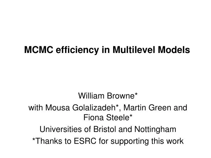
MCMC efficiency in Multilevel Models. William Browne* with Mousa Golalizadeh*, Martin Green and Fiona Steele* Universities of Bristol and Nottingham *Thanks to ESRC for supporting this work. Summary. Introduction. Application 1 – Clutch size in great tits. Method 1: Hierarchical centering.

E N D
MCMC efficiency in Multilevel Models William Browne* with Mousa Golalizadeh*, Martin Green and Fiona Steele* Universities of Bristol and Nottingham *Thanks to ESRC for supporting this work
Summary • Introduction. • Application 1 – Clutch size in great tits. • Method 1: Hierarchical centering. • Method 2: Parameter expansion. • Application 2 – Mastitis incidence in dairy cattle. • Method 3: Orthogonal predictors. • Application 3 – Contraceptive discontinuation in Indonesia. • Conclusions. • Further Work.
Introduction/Synopsis • MCMC methods allow easy fitting of complex random effects models • The simplest (default) MCMC algorithms can produce poorly mixing chains. • By reparameterising the model one can greatly improve mixing. • These reparameterisations are easy to implement in WinBUGS (or MLwiN) • The choice of reparameterisation depends in part on the model/dataset.
Application 1: Great tit nesting behaviour (crossed random effects) • Original work was collaborative research with Richard Pettifor (Institute of Zoology, London), and Robin McCleery and Ben Sheldon (University of Oxford).
Application 1: Great tit nesting behaviour (crossed random effects) • A longitudinal study of great tits nesting in Wytham Woods, Oxfordshire. • 6 responses : 3 continuous & 3 binary. • Clutch size, lay date and mean nestling mass. • Nest success, male and female survival. • Data: 4165 nesting attempts over a period of 34 years. • There are 4 higher-level classifications of the data: female parent, male parent, nestbox and year. • We only consider Clutch size here
Source Number of IDs Median #obs Mean #obs Year 34 104 122.5 Nestbox 968 4 4.30 Male parent 2986 1 1.39 Female parent 2944 1 1.41 Data background The data structure can be summarised as follows: Note there is very little information on each individual male and female bird but we can get some estimates of variability via a random effects model.
MCMC efficiency for clutch size response • The MCMC algorithm used in the univariate analysis of clutch size was a simple 10-step Gibbs sampling algorithm. • . • To compare methods for each parameter we can look at the effective sample sizes (ESS) which give an estimate of how many ‘independent samples we have’ for each parameter as opposed to 50,000 dependent samples. • ESS = # of iterations/,
Parameter MLwiN WinBUGS Fixed Effect 671 602 Year 30632 29604 Nestbox 833 788 Male 36 33 Female 3098 3685 Observation 110 135 Time 519s 2601s Effective Sample sizes We will now consider methods that will improve the ESS values for particular parameters. We will firstly consider the fixed effect parameter.
Trace and autocorrelation plots for fixed effect using standard Gibbs sampling algorithm
Hierarchical Centering This method was devised by Gelfand et al. (1995) for use in nested models. Basically (where feasible) parameters are moved up the hierarchy in a model reformulation. For example: is equivalent to The motivation here is we remove the strong negative correlation between the fixed and random effects by reformulation.
Hierarchical Centering In our cross-classified model we have 4 possible hierarchies up which we can move parameters. We have chosen to move the fixed effect up the year hierarchy as it’s variance had biggest ESS although this choice is rather arbitrary. The ESS for the fixed effect increases 50-fold from 602 to 35,063 while for the year level variance we have a smaller improvement from 29,604 to 34,626. Note this formulation also runs faster 1864s vs 2601s (in WinBUGS).
Trace and autocorrelation plots for fixed effect using hierarchical centering formulation
Parameter Expansion • We next consider the variances and in particular the between-male bird variance. • When the posterior distribution of a variance parameter has some mass near zero this can hamper the mixing of the chains for both the variance parameter and the associated random effects. • The pictures over the page illustrate such poor mixing. • One solution is parameter expansion (Liu et al. 1998). • In this method we add an extra parameter to the model to improve mixing.
Trace plots for between males variance and a sample male effect using standard Gibbs sampling algorithm
Parameter Expansion In our example we use parameter expansion for all 4 hierarchies. Note the parameters have an impact on both the random effects and their variance. The original parameters can be found by: Note the models are not identical as we now have different prior distributions for the variances.
Parameter Expansion • For the between males variance we have a 20-fold increase in ESS from 33 to 600. • The parameter expanded model has different prior distributions for the variances although these priors are still ‘diffuse’. • It should be noted that the point and interval estimate of the level 2 variance has changed from • 0.034 (0.002,0.126) to 0.064 (0.000,0.172). • Parameter expansion is computationally slower 3662s vs 2601s for our example.
Trace plots for between males variance and a sample male effect using parameter expansion.
Combining the two methods Hierarchical centering and parameter expansion can easily be combined in the same model. Here we perform centering on the year classification and parameter expansion on the other 3 hierarchies.
Parameter WinBUGS originally WinBUGS combined Fixed Effect 602 34296 Year 29604 34817 Nestbox 788 5170 Male 33 557 Female 3685 8580 Observation 135 1431 Time 2601s 2526s Effective Sample sizes As we can see below the effective sample sizes for all parameters are improved for this formulation while running time remains approximately the same.
Application 2: Contraceptive discontinuation in Indonesia • Steele et al. (2004) use multilevel multistate models to study transitions in and out of contraceptive use in Indonesia. Here we consider a simplification of their model which considers only the transition from use to non-use, commonly referred to as contraceptive discontinuation. • The data come from the 1997 Indonesia Demographic and Health Survey. Contraceptive use histories were collected retrospectively for the six-year period prior to the survey, and include information on the month and year of starting and ceasing use, the method used, and the reason for discontinuation. • The analysis is based on 17,833 episodes of contraceptive use for 12,594 women, where an episode is defined as a continuous period of using the same method of contraception. • Restructuring the data to discrete-time format with monthly time intervals leads to 365,205 records. To reduce the size, monthly intervals are grouped into six-month intervals and a binomial response is defined with denominator equal to the number of months of use within a six-month interval. Aggregation of intervals leads to a dataset with 68,515 records.
Model • We here have intervals nested within episodes nested within women. Here we include discrete categories for the duration terms zt – a piecewise constant hazard with categories representing 6-11 months, 12-23 months, 24-35 months and >35 months with a base category of 0-5 months.
Predictors • At the episode level we have: Age categorized as <25,25-34 and 34-49. Contraceptive method categorized as pill/injectable, Norplant/IUD, other modern and traditional. • At the woman level we have: Education (3 categories). Type of region of residence (urban/rural). Socioeconomic status (low, medium or high).
Results The table below gives the effective sample sizes based on runs of 250,000 iterations. Here the hierarchical centered formulation does really badly. This is because the cluster variance σ2u is very small: estimates of 0.041 and 0.022 for the two methods
A closer look at the residuals • It is well known that hierarchical centering works best if the cluster level variance is substantial. • Here we see that both the variance is small and the distribution of the residuals is not very normal. • This is due to a few women who discontinue usage very quickly and often, whilst many women never discontinue! Std residuals Normal scores
Simple logistic regression • We will consider first removing the random effects from the model (due to their small variance) which will result in a simple logistic regression model. • It will then be impossible to perform hierarchical centering however we will consider the use of orthogonalisation. • Note that Hills and Smith (1992) talk about using orthogonal parameterisations and Roberts and Gilks give it one sentence in ‘MCMC in Practice’. Here we consider it in combination with the simple (single site) random walk Metropolis sampler where reduction of correlation in the posterior is perhaps most important.
Method 3:Orthogonal parameterisation • For simplicity assume we have all predictors in one matrix P and that we can write ztα+xtijβ as ptijθ where θ=(α,β). • Step 1: Number the predictors in some ordering 1,…,N. • Step 2: Take each predictor in turn and replace it with a predictor that is orthogonal to all the already considered predictors. • For predictor pk. • Note this requires solving k-1 equations in k-1 unknown w parameters. • A different orthogonal set of predictors results from each ordering.
Orthogonal parameterisation • The second step of the algorithm produces both a set of orthogonal predictors that span the same space as the original predictors and a group of w coefficients that can be combined to form a lower diagonal matrix W. • We can fit this model and recover the coefficients for the original predictors by pre-multiplication by WT. • It is worth noting here that we use improper Uniform priors for the coefficients and if we used proper priors we would need to also calculate the Jacobian for the reparameterisation to ensure the same priors are used. • We ordered the predictors in what follows so that the level 2 predictors were last before performing reparameterisation.
Results • The following is based on 50,000 iterations: Here we see almost universal benefit of the orthogonal parameterisation with virtually zero time costs and very little programming!
Combining orthogonalisation with parameter expansion • Combining orthogonalisation and parameter expansion we have: We ran this model using WinBUGS and only 25,000 iterations following a burnin of 500 iterations which took 34 hours compared to 23½ for 250k in MLwiN without parameter expansion. The results are given overleaf.
Results for full model • Here we compare simply using the orthogonal approach in MLwiN for 250k with both orthogonal predictors and parameter expansion in WinBUGS for 25k. Note this takes ~1.5 times as long:
Trace plots of variance chain Here we see the far greater mixing of the variance chain after parameter expansion. It is worth noting that parameter expansion uses a different prior for σ2u and results in an estimate of 0.059 (0.048) as opposed to 0.008 (0.006) without and earlier estimates of 0.041(0.026) and 0.022 (0.018) before orthogonalisation. Note however that all estimates bar parameter expansion are based on very low ESS! Before Parameter Expansion After Parameter Expansion
Conclusions • Hierarchical centering – as is well known - works well when the cluster variance is big but is no good for small variances • Other research building on hierarchical centering includes Papaspiliopoulus et al. (2003,2007) showing how to construct partially non-centred parameterisations. • Parameter expansion works well to improve mixing when the cluster variance is small but results in a different prior for the variance. • Orthogonalisation of predictors appears to be a good idea generally but is slightly more involved than the other reparameterisations i.e. the predictors need orthogonalising outside WinBUGS and the chains need transforming back. • An interesting area of further research is choosing the order for orthogonalisation i.e. which set of orthogonal predictors to use.
Current Work • E-STAT node in the ESRC funded NCeSS program began in September 2009 including researchers from Bristol, Southampton, Manchester, IOE and Stirling. • Software to cater for all types of users including novice practitioners, advanced practitioners and software developers. • Based around a new algebraic processing system and MCMC engine written in Python but also includes interoperability with other packages. • A series of model templates for specific model families are being developed with the idea being that advanced users develop their own (domain specific) templates. • A browser based user interface is being developed. • Website: http://www.cmm.bristol.ac.uk/research/NCESS-EStat/ or see me for a demonstration of current version.
References • Browne, W.J. (2003). MCMC Estimation in MLwiN. London: Institute of Education, University of London • Browne, W.J. (2004). An illustration of the use of reparameterisation methods for improving MCMC efficiency in crossed random effect models Multilevel Modelling Newsletter 16 (1): 13-25 • Browne, W.J., Steele F., Golalizadeh, M., and Green M.J. (2009) The use of simple reparameterizations to improve the efficiency of Markov chain Monte Carlo estimation for multilevel models with applications to discrete time survival models Journal of Royal Statistical Society, Series A. 172: 579-598 • Gamerman D. (1997) Sampling from the posterior distribution in generalized linear mixed models. Statistics and Computing. 7, 57--68. • Gelfand, A.E., Sahu, S.K. and Carlin, B.P. (1995) Efficient parameterisations for normal linear mixed models. Biometrika 83, 479--488 • Gelman, A., Huang, Z., van Dyk, D., and Boscardin, W.J. (2007). Using redundant parameterizations to fit hierarchical models. Journal of Computational and Graphical Statistics (to appear). • Hills, S.E. and Smith, A.F.M. (1992) Parameterization Issues in Bayesian Inference. In Bayesian Statistics 4, (J M Bernardo, J O Berger, A P Dawid, and A F M Smith, eds), Oxford University Press, UK, pp. 227--246.
References cont. • Liu, C., Rubin, D.B., and Wu, Y.N. (1998) Parameter expansion to accelerate EM: The PX-EM algorithm. Biometrika 85 (4): 755-770. • Liu, J.S., Wu, Y.N. (1999) Parameter Expansion for Data Augmentation. Journal Of The American Statistical Association 94: 1264-1274 • Papaspiliopoulos, O, Roberts, G.O. and Skold, M. (2003) Non-centred Parameterisations for Hierarchical Models and Data Augmentation. In Bayesian Statistics 7, (J M Bernardo, M J Bayarri, J O Berger, A P Dawid, D Heckerman, A F M Smith and M West, eds), Oxford University Press, UK, pp. 307--32 • Papaspiliopoulos, O, Roberts, G.O. and Skold, M. (2007) A General Framework for the Parametrization of Hierarchical Models. Statistical Science 22, 59--73. • Rasbash, J., Browne, W.J., Healy, M, Cameron, B and Charlton, C. (2000). The MLwiN software package version 1.10. London: Institute of Education, University of London. • Steele, F., Goldstein, H. and Browne, W.J. (2004). A general multilevel multistate competing risks model for event history data, with an application to a study of contraceptive use dynamics. Statistical Modelling 4: 145--159 • Van Dyk, D.A., and Meng, X-L. (2001) The Art of Data Augmentation. Journal of Computational and Graphical Statistics. 10, 1--50.