Download
1 / 49
500 likes | 774 Views
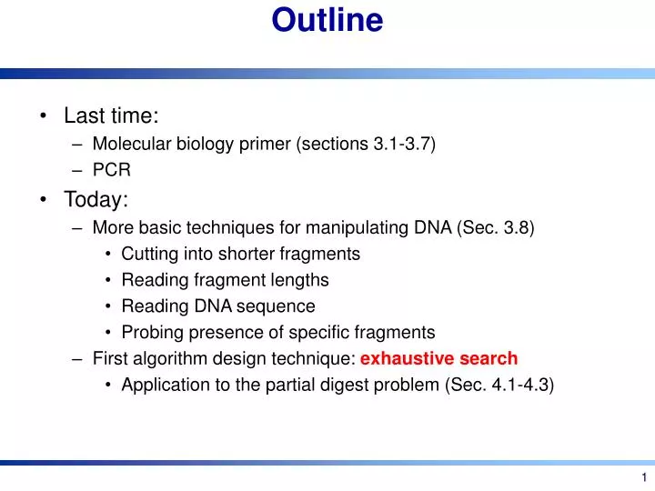
Outline. Last time: Molecular biology primer (sections 3.1-3.7) PCR Today: More basic techniques for manipulating DNA (Sec. 3.8) Cutting into shorter fragments Reading fragment lengths Reading DNA sequence Probing presence of specific fragments

E N D
Outline • Last time: • Molecular biology primer (sections 3.1-3.7) • PCR • Today: • More basic techniques for manipulating DNA (Sec. 3.8) • Cutting into shorter fragments • Reading fragment lengths • Reading DNA sequence • Probing presence of specific fragments • First algorithm design technique: exhaustive search • Application to the partial digest problem (Sec. 4.1-4.3)
Restriction Enzymes • Discovered in the early 1970’s • Used as a defense mechanism by bacteria to break down the DNA of attacking viruses. • They cut the DNA into small fragments. • Can also be used to cut the DNA of organisms. • This allows the DNA sequence to be in a more manageable bite-size pieces. • It is then possible using standard purification techniques to single out certain fragments and duplicate them to macroscopic quantities.
Molecular Scissors Molecular Cell Biology, 4th editionfig 9-10
Separating DNA by Size • Gel Electrophoresis • DNA fragments are injected into a gel positioned in an electric field • DNA is negatively charged near neutral pH DNA molecules move towards the positive electrode • Smaller molecules move through the gel matrix faster than larger molecules • The gel matrix restricts random diffusion so molecules of different lengths separate into bands
Detecting DNA • Autoradiography • The DNA is radioactively labeled • The gel is laid against a sheet of photographic film in the dark, exposing the film at the positions where the DNA is present • Fluorescence • The gel is incubated with a solution containing the fluorescent dye ethidium • Ethidium binds to the DNA • The DNA lights up when the gel is exposed to ultraviolet light
Gel Electrophoresis: Example Direction of DNA movement Smaller fragments travel farther
Sequencing • Biologists can reliably find the sequence of A/C/T/G for short strings (few hundred nucleotides) • Chain termination • Single strand template • Complementary strand synthesis blocked with small probability at particular nucleotides • Lengths of fragments read for each class of strings
Sequencing • Chain termination (See animation) • PCR-like reaction • Single primer • Complementary strand synthesis is blocked with small probability at particular nucleotides (A/C/T/G) • Lengths of fragments read for each class of strings
DNA Microarrays • Exploit Watson-Crick complementarity to simultaneously perform a large number of substring tests • Used in a variety of genomic analyses • Transcription (gene expression) analysis • Single Nucleotide Polymorphism (SNP) genotyping • Genomic-based microorganism identification • Common microarray formats involve direct hybridization between labeled DNA/RNA sample and DNA probes attached to a glass slide
Labeled DNA/RNA sample hybridized to array of probes Laser activation of fluorescent labels Optical scanning used to identify probes with complements in the mixture Direct Hybridization Experiment Images courtesy of Affymetrix.
cell type 1 RNA 1 target 1 Cy3 Cy3 Cy3 target 2 Cy5 Cy5 Cy5 RNA 2 cell type 2 Two-Color Technique • Sample labeled RED • Control labeled GREEN • YELLOW probes hybridize to both sample and control • BLACK probes hybridize to neither
Restriction Maps • A map of all restriction sites in a DNA sequence • Can be constructed through both biological and computational methods without knowing DNA sequence
Full Restriction Digest • Cutting DNA at each restriction site creates • multiple restriction fragments: • Is it possible to reconstruct the order of the fragments and the positions of the cuts?
Full Restriction Digest: Multiple Solutions • An alternative ordering of restriction fragments: vs
Partial Restriction Digest • The sample of DNA is exposed to the restriction enzyme for only a limited amount of time to prevent it from being cut at all restriction sites • We assume that with this method biologists can generate the set of all possible restriction fragments between every two cuts • We assume that multiplicity of a fragment can be detected, i.e., the number of restriction fragments of the same length can be determined (e.g., by observing twice as much fluorescence intensity for a double fragment than for a single fragment) • This set of fragment sizes is used to determine the positions of the restriction sites in the DNA sequence
Partial Digest Example • For the same DNA sequence as before, we would now get the following restriction fragments:
Partial Digest Fundamentals Defining some of the terms used in the Partial Digest Problem: X: the set of n integers representing the location of all cuts in the restriction map, including the start and end n: the total number of cuts X: the multiset of integers representing lengths of each of the fragments produced from a partial digest
One More Partial Digest Example Representation of X= {2, 2, 3, 3, 4, 5, 6, 7, 8, 10} as a two dimensional table, with elements of X = {0, 2, 4, 7, 10} along both the top and left side. The elements at (i, j) in the table is the value xi – xj for 1 ≤ i < j ≤ n.
Partial Digest Problem: Formulation Partial Digest Problem: Given all pairwise distances between points on a line, reconstruct the positions of those points • Input: The multiset of pairwise distances L, containing integers • Output: A set X, of n integers, such that X = L
Partial Digest: Multiple Solutions • It is not always possible to uniquely reconstruct a set X based only on X • Sets {0,1,2,5,7,9,12} and {0,1,5,7,8,10,12} both produce partial digest set {1, 1, 2, 2, 2, 3, 3, 4, 4, 5, 5, 5, 6, 7, 7, 7, 8, 9, 10, 11, 12}
Exhaustive Search Algorithms • Also known as brute force algorithms; examine every possible solution until you find a valid one • (e.g., list sorting): look at all permutations of elements in the list until finding the sorted version • Usually impractical!
Partial Digest: Brute Force • Find the restriction fragment of maximum length M. M is the length of the DNA sequence. • For every possible solution, compute the corresponding X • If X is equal to the experimental partial digest L, then X is the correct restriction map
BruteForcePDP • BruteForcePDP(L, n): • M maximum element in L • for every set of n – 2 integers 0 < x2 < … xn-1 < M • X {0,x2,…,xn-1,M} • Form Xfrom X • ifX=L • return X • output “no solution”
Efficiency of BruteForcePDP • The speed of the BruteForceDPD is unfortunately O(Mn-2) as it must examine all possible sets of positions. • One way to improve the algorithm is to limit the values of xi to only those values which occur in L
AnotherBruteForcePDP • AnotherBruteForcePDP(L, n) • M maximum element in L • for every set of n – 2 integers 0 < x2 < … xn-1 < Mfrom L • X { 0,x2,…,xn-1,M} • Form Xfrom X • if X=L • return X • output “no solution”
Efficiency of AnotherBruteForcePDP • It’s more efficient, but still slow • Only sets examined, but runtime is still exponential: O(n2n-4) • If L = {2, 998, 1000} (n = 3, M= 1000), BruteForcePDP will be extremely slow, but AnotherBruteForcePDP will be quite fast
Branch and Bound Algorithm for PDP • Begin with X = {0} • Remove the largest element in L and place it in X • See if the element fits on the right or left side of the restriction map • When it fits, find the other lengths it creates and remove those from L • Go back to step 1 until L is empty
An Example L = { 2, 2, 3, 3, 4, 5, 6, 7, 8, 10 } X = { 0 }
An Example L = { 2, 2, 3, 3, 4, 5, 6, 7, 8, 10 } X = { 0 } Remove 10 from L and insert it into X. We know this must be the length of the DNA sequence because it is the largest fragment.
An Example L = { 2, 2, 3, 3, 4, 5, 6, 7, 8, 10 } X = { 0, 10 }
An Example L = { 2, 2, 3, 3, 4, 5, 6, 7, 8, 10 } X = { 0, 10 } Take 8 from L and make y = 2 or 8. But since the two cases are symmetric, we can assume y = 2. We find that the distances from y to other elements at X are (y, X) = {8, 2}, so we remove {8, 2} from L and add 2 to X. (y, X) = {|y – x1|, |y – x2|, …, |y – xn|} forX = {x1, x2, …, xn}
An Example L = { 2, 2, 3, 3, 4, 5, 6, 7, 8, 10 } X = { 0, 2, 10 }
An Example L = { 2, 2, 3, 3, 4, 5, 6, 7, 8, 10 } X = { 0, 2, 10 } Take 7 from L and make y = 7 or y = 10 – 7 = 3. We will explore y = 7 first, so (y, X ) = {7, 5, 3}. Therefore we remove {7, 5 ,3} from L and add 7 to X. (y, X) = {7, 5, 3} = {7 – 0, 7 – 2, 7 – 10}
An Example L = { 2, 2, 3, 3, 4, 5, 6, 7, 8, 10 } X = { 0, 2, 7, 10 }
6 An Example L = { 2, 2, 3, 3, 4, 5, 6, 7, 8, 10 } X = { 0, 2, 7, 10 } Take 6 from L and make y = 6. Unfortunately (y, X) = {6, 4, 1 ,4}, which is not a subset of L. Therefore we won’t explore this branch.
An Example L = { 2, 2, 3, 3, 4, 5, 6, 7, 8, 10 } X = { 0, 2, 7, 10 } This time make y = 4. (y, X) = {4, 2, 3 ,6}, which is a subset of L so we will explore this branch. We remove {4, 2, 3 ,6} from L and add 4 to X.
An Example L = { 2, 2, 3, 3, 4, 5, 6, 7, 8, 10 } X = { 0, 2, 4, 7, 10 }
An Example L = { 2, 2, 3, 3, 4, 5, 6, 7, 8, 10 } X = { 0, 2, 4, 7, 10 } L is now empty, so we have a solution, which is X.
An Example L = { 2, 2, 3, 3, 4, 5, 6, 7, 8, 10 } X = { 0, 2, 7, 10 } To find other solutions, we backtrack.
An Example L = { 2, 2, 3, 3, 4, 5, 6, 7, 8, 10 } X = { 0, 2, 10 } More backtrack.
An Example L = { 2, 2, 3, 3, 4, 5, 6, 7, 8, 10 } X = { 0, 2, 10 } This time we will explore y = 3. (y, X) = {3, 1, 7}, which is not a subset of L, so we won’t explore this branch.
An Example L = { 2, 2, 3, 3, 4, 5, 6, 7, 8, 10 } X = { 0, 10 } We backtracked back to the root. Therefore we have found all the solutions.
Analyzing PartialDigest Algorithm • Still exponential in worst case, but is very fast on average • For n different fragments, if time of PartialDigest is T(n): • No branching case: T(n) < T(n-1) + O(n) • Quadratic • Branching case: T(n) < 2T(n-1) + O(n) • Exponential
Double Digest Mapping • Double Digest is experimentally simpler method than Partial Digest to generate data for a restriction map • Use two restriction enzymes; three full digests: • One with only first enzyme • One with only second enzyme • One with both enzymes • Computationally more complex to figure out than partial digest problem
Double Digest Problem Input: A – the set of fragment lengths from the digest with first restriction enzyme A. B – the set of fragment lengths from the digest with second restriction enzyme B. X – the set of fragment lengths from the digest with both restriction enzymes A and B. Output: A– location of the cuts in the restriction map for the first restriction enzyme. B – location of the cuts in the restriction map for the second restriction enzyme. Note: X = A B and X contains 0 and t with 0 A, B and t A, B.
Double Digest: Example Without the information about X (i.e.A+B), it is impossible to solve the double digest problem as this diagram illustrates