Download
1 / 17
170 likes | 328 Views
Quantifying spatial patterns of transpiration in xeric and mesic forests. Jonathan D. Adelman 1 Brent E. Ewers 1 Mike Loranty 2 D. Scott Mackay 2 June 1, 2005 1: University of Wyoming 2: SUNY Buffalo. Cookie-cutter approach vs. spatially explicit upscaling.

E N D
Quantifying spatial patternsof transpiration in xericand mesic forests Jonathan D. Adelman 1 Brent E. Ewers 1 Mike Loranty 2 D. Scott Mackay 2 June 1, 2005 1: University of Wyoming 2: SUNY Buffalo
Cookie-cutter approachvs. spatially explicit upscaling -Traditional means of quantifying carbon and water fluxes have not been spatially explicit. -Some ChEAS-based studies have successfully utilized this approach; however, changes in site gradient or management plan would have likely rendered traditional sampling ineffective. EC = canopy transpiration JS = sap flux AS:AG = sap wood to ground area ratio KL = hydraulic conductance ΨS = soil water potential ΨL = leaf water potential GS = canopy stomatal conductance LAI = leaf area index VPD = vapor pressure deficit Traditional method: pick one point in a stand, measure parameter(s) of interest, and assume the rest of the stands exhibits identical behavior. EC=JS·(AS:AG) EC=KL·(ΨS-ΨL) EC=GS·LAI·(VPD)
Cookie-cutter approachvs. spatially explicit upscaling -Geostatistical analyses appearing more often in ecology literature. -Rarely used with flux ecology, mostly with soils; no prominent studies quantify ecophysiological spatial patterns. -Water is easy to measure spatially; is continuous; good eventual proxy for carbon fluxes. EC = canopy transpiration JS = sap flux AS:AG = sap wood to ground area ratio KL = hydraulic conductance ΨS = soil water potential ΨL = leaf water potential GS = canopy stomatal conductance LAI = leaf area index VPD = vapor pressure deficit Spatially explicit method: allow parameter to vary across the stand. EC=JS·(AS:AG) EC=KL·(ΨS-ΨL) EC=GS·LAI·(VPD)
Traditional geostatistical analyses The semivariance of a measured parameter (in this case, soil moisture) is used to create a kriged surface. This methodology can also be used with flux measurements.
Objectives • Determine whether spatial patterns of transpiration exist • If not spatial patterns exist, use cookie-cutter approach • If spatial patterns exist, models must be spatially explicit • Determine whether spatial patterns change in time • Determine whether spatial patterns change with scaling • Determine whether spatial patterns change across ecosystems • If so, easily measured proxy is needed • Test methodology in two differing ecosystems • Wisconsin: mesic site, lowland upland gradient • Wyoming: xeric site, low-lying creek hilltop gradient
Wetland Low slope Transition Mid slope Upland High slope Study sites Wisconsin Wyoming -moisture gradients -VPD -sap flux -soil moisture -VPD 120m x 120m area 80m x 184m area
The semi-variogram c g = semi-variance distance = distance between point pairs a = sill b = range c = nugget
Semi-variograms of VPDand soil moisture July 28, 2004 August 5, 2004
Conclusions • Spatial patterns of sap flux and transpiration exist: • models must be spatially explicit, OR • easily measurable proxies must be found • Spatial patterns of sap flux and transpiration change: • across time • across ecosystems • with upscaling • Implications for carbon flux measurements • Proxies: • remotely sensed imagery • physiological parameters such as LAI
Acknowledgements Wisconsin-based research has been funded by NSF Hydrologic Sciences (EAR-0405306 to D.S. Mackay, EAR-0405381 to B.E. Ewers, and EAR-0405318 to E.L. Kruger). Wyoming-based research has been funding by Wyoming NASA Space Grant Consortium’s 2004 Graduate Research Fellowship (to J.D. Adelman). Thanks to the Principal Investigators, as well as Mike Loranty, Erin Loranty, and Tim Wert for assistance at the ChEAS study site, and Mel Durrett and Ian Abernethy for assistance at the Snowy Range study site. Special thanks to Sarah Kerker, whose fingerprints have left indelible marks at both sites.