Download
1 / 98
1.02k likes | 1.67k Views
Option Pricing Theory and Real Option Applications. Aswath Damodaran. What is an option?.

E N D
Option Pricing Theory and Real Option Applications Aswath Damodaran
What is an option? • An option provides the holder with the right to buy or sell a specified quantity of an underlying asset at a fixed price (called a strike price or an exercise price) at or before the expiration date of the option. • Since it is a right and not an obligation, the holder can choose not to exercise the right and allow the option to expire. • There are two types of options - call options (right to buy) and put options (right to sell).
Call Options • A call option gives the buyer of the option the right to buy the underlying asset at a fixed price (strike price or K) at any time prior to the expiration date of the option. The buyer pays a price for this right. • At expiration, • If the value of the underlying asset (S) > Strike Price(K) • Buyer makes the difference: S - K • If the value of the underlying asset (S) < Strike Price (K) • Buyer does not exercise • More generally, • the value of a call increases as the value of the underlying asset increases • the value of a call decreases as the value of the underlying asset decreases
Payoff Diagram on a Call Net Payoff on Call Strike Price Price of underlying asset
Put Options • A put option gives the buyer of the option the right to sell the underlying asset at a fixed price at any time prior to the expiration date of the option. The buyer pays a price for this right. • At expiration, • If the value of the underlying asset (S) < Strike Price(K) • Buyer makes the difference: K-S • If the value of the underlying asset (S) > Strike Price (K) • Buyer does not exercise • More generally, • the value of a put decreases as the value of the underlying asset increases • the value of a put increases as the value of the underlying asset decreases
Payoff Diagram on Put Option Net Payoff On Put Strike Price Price of underlying asset
Determinants of option value • Variables Relating to Underlying Asset • Value of Underlying Asset; as this value increases, the right to buy at a fixed price (calls) will become more valuable and the right to sell at a fixed price (puts) will become less valuable. • Variance in that value; as the variance increases, both calls and puts will become more valuable because all options have limited downside and depend upon price volatility for upside. • Expected dividends on the asset, which are likely to reduce the price appreciation component of the asset, reducing the value of calls and increasing the value of puts. • Variables Relating to Option • Strike Price of Options; the right to buy (sell) at a fixed price becomes more (less) valuable at a lower price. • Life of the Option; both calls and puts benefit from a longer life. • Level of Interest Rates; as rates increase, the right to buy (sell) at a fixed price in the future becomes more (less) valuable.
American versus European options: Variables relating to early exercise • An American option can be exercised at any time prior to its expiration, while a European option can be exercised only at expiration. • The possibility of early exercise makes American options more valuable than otherwise similar European options. • However, in most cases, the time premium associated with the remaining life of an option makes early exercise sub-optimal. • While early exercise is generally not optimal, there are two exceptions: • One is where the underlying asset pays large dividends, thus reducing the value of the asset, and of call options on it. In these cases, call options may be exercised just before an ex-dividend date, if the time premium on the options is less than the expected decline in asset value. • The other is when an investor holds both the underlying asset and deep in-the-money puts on that asset, at a time when interest rates are high. The time premium on the put may be less than the potential gain from exercising the put early and earning interest on the exercise price.
A Summary of the Determinants of Option Value Factor Call Value Put Value Increase in Stock Price Increases Decreases Increase in Strike Price Decreases Increases Increase in variance of underlying asset Increases Increases Increase in time to expiration Increases Increases Increase in interest rates Increases Decreases Increase in dividends paid Decreases Increases
Creating a replicating portfolio • The objective in creating a replicating portfolio is to use a combination of riskfree borrowing/lending and the underlying asset to create the same cashflows as the option being valued. • Call = Borrowing + Buying D of the Underlying Stock • Put = Selling Short D on Underlying Asset + Lending • The number of shares bought or sold is called the option delta. • The principles of arbitrage then apply, and the value of the option has to be equal to the value of the replicating portfolio.
The Limiting Distributions…. • As the time interval is shortened, the limiting distribution, as t -> 0, can take one of two forms. • If as t -> 0, price changes become smaller, the limiting distribution is the normal distribution and the price process is a continuous one. • If as t->0, price changes remain large, the limiting distribution is the poisson distribution, i.e., a distribution that allows for price jumps. • The Black-Scholes model applies when the limiting distribution is the normal distribution , and explicitly assumes that the price process is continuous and that there are no jumps in asset prices.
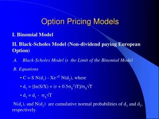
The Black-Scholes Model • The version of the model presented by Black and Scholes was designed to value European options, which were dividend-protected. • The value of a call option in the Black-Scholes model can be written as a function of the following variables: S = Current value of the underlying asset K = Strike price of the option t = Life to expiration of the option r = Riskless interest rate corresponding to the life of the option 2 = Variance in the ln(value) of the underlying asset
The Black Scholes Model Value of call = S N (d1) - K e-rt N(d2) where, • d2 = d1 - √t • The replicating portfolio is embedded in the Black-Scholes model. To replicate this call, you would need to • Buy N(d1) shares of stock; N(d1) is called the option delta • Borrow K e-rt N(d2)
Adjusting for Dividends • If the dividend yield (y = dividends/ Current value of the asset) of the underlying asset is expected to remain unchanged during the life of the option, the Black-Scholes model can be modified to take dividends into account. C = S e-yt N(d1) - K e-rt N(d2) where, d2 = d1 - √t • The value of a put can also be derived: P = K e-rt (1-N(d2)) - S e-yt (1-N(d1))
Problems with Real Option Pricing Models 1. The underlying asset may not be traded, which makes it difficult to estimate value and variance for the underlying asset. 2. The price of the asset may not follow a continuous process, which makes it difficult to apply option pricing models (like the Black Scholes) that use this assumption. 3. The variance may not be known and may change over the life of the option, which can make the option valuation more complex. 4. Exercise may not be instantaneous, which will affect the value of the option. 5. Some real options are complex and their exercise creates other options (compound) or involve learning (learning options)
Option Pricing Applications in Investment/Strategic Analysis
Options in Projects/Investments/Acquisitions • One of the limitations of traditional investment analysis is that it is static and does not do a good job of capturing the options embedded in investment. • The first of these options is the option to delay taking a investment, when a firm has exclusive rights to it, until a later date. • The second of these options is taking one investment may allow us to take advantage of other opportunities (investments) in the future • The last option that is embedded in projects is the option to abandon a investment, if the cash flows do not measure up. • These options all add value to projects and may make a “bad” investment (from traditional analysis) into a good one.
The Option to Delay • When a firm has exclusive rights to a project or product for a specific period, it can delay taking this project or product until a later date. • A traditional investment analysis just answers the question of whether the project is a “good” one if taken today. • Thus, the fact that a project does not pass muster today (because its NPV is negative, or its IRR is less than its hurdle rate) does not mean that the rights to this project are not valuable.
Valuing the Option to Delay a Project PV of Cash Flows from Project Initial Investment in Project Present Value of Expected Cash Flows on Product Project's NPV turns Project has negative positive in this section NPV in this section
Insights for Investment Analyses • Having the exclusive rights to a product or project is valuable, even if the product or project is not viable today. • The value of these rights increases with the volatility of the underlying business. • The cost of acquiring these rights (by buying them or spending money on development, for instance) has to be weighed off against these benefits.
Example 1: Valuing product patents as options • A product patent provides the firm with the right to develop the product and market it. • It will do so only if the present value of the expected cash flows from the product sales exceed the cost of development. • If this does not occur, the firm can shelve the patent and not incur any further costs. • If I is the present value of the costs of developing the product, and V is the present value of the expected cashflows from development, the payoffs from owning a product patent can be written as: Payoff from owning a product patent = V - I if V> I = 0 if V ≤ I
Payoff on Product Option Net Payoff to introduction Cost of product introduction Present Value of cashflows on product
Valuing a Product Patent: Avonex • Biogen, a bio-technology firm, has a patent on Avonex, a drug to treat multiple sclerosis, for the next 17 years, and it plans to produce and sell the drug by itself. The key inputs on the drug are as follows: PV of Cash Flows from Introducing the Drug Now = S = $ 3.422 billion PV of Cost of Developing Drug for Commercial Use = K = $ 2.875 billion Patent Life = t = 17 years Riskless Rate = r = 6.7% (17-year T.Bond rate) Variance in Expected Present Values =s2 = 0.224 (Industry average firm variance for bio-tech firms) Expected Cost of Delay = y = 1/17 = 5.89% d1 = 1.1362 N(d1) = 0.8720 d2 = -0.8512 N(d2) = 0.2076 Call Value= 3,422 exp(-0.0589)(17) (0.8720) - 2,875 (exp(-0.067)(17) (0.2076)= $ 907 million
Valuing a firm with patents • The value of a firm with a substantial number of patents can be derived using the option pricing model. Value of Firm = Value of commercial products (using DCF value + Value of existing patents (using option pricing) + (Value of New patents that will be obtained in the future – Cost of obtaining these patents) • The last input measures the efficiency of the firm in converting its R&D into commercial products. If we assume that a firm earns its cost of capital from research, this term will become zero. • If we use this approach, we should be careful not to double count and allow for a high growth rate in cash flows (in the DCF valuation).
Value of Biogen’s existing products • Biogen had two commercial products (a drug to treat Hepatitis B and Intron) at the time of this valuation that it had licensed to other pharmaceutical firms. • The license fees on these products were expected to generate $ 50 million in after-tax cash flows each year for the next 12 years. To value these cash flows, which were guaranteed contractually, the pre-tax cost of debt of 7% of the licensing firms was used: Present Value of License Fees = $ 50 million (1 – (1.07)-12)/.07 = $ 397.13 million
Value of Biogen’s Future R&D • Biogen continued to fund research into new products, spending about $ 100 million on R&D in the most recent year. These R&D expenses were expected to grow 20% a year for the next 10 years, and 5% thereafter. • It was assumed that every dollar invested in research would create $ 1.25 in value in patents (valued using the option pricing model described above) for the next 10 years, and break even after that (i.e., generate $ 1 in patent value for every $ 1 invested in R&D). • There was a significant amount of risk associated with this component and the cost of capital was estimated to be 15%.
Value of Future R&D Yr Value of R&D Cost Excess Value Present Value Patents (at 15%) 1 $ 150.00 $ 120.00 $ 30.00 $ 26.09 2 $ 180.00 $ 144.00 $ 36.00 $ 27.22 3 $ 216.00 $ 172.80 $ 43.20 $ 28.40 4 $ 259.20 $ 207.36 $ 51.84 $ 29.64 5 $ 311.04 $ 248.83 $ 62.21 $ 30.93 6 $ 373.25 $ 298.60 $ 74.65 $ 32.27 7 $ 447.90 $ 358.32 $ 89.58 $ 33.68 8 $ 537.48 $ 429.98 $ 107.50 $ 35.14 9 $ 644.97 $ 515.98 $ 128.99 $ 36.67 10 $ 773.97 $ 619.17 $ 154.79 $ 38.26 $ 318.30
Value of Biogen • The value of Biogen as a firm is the sum of all three components – the present value of cash flows from existing products, the value of Avonex (as an option) and the value created by new research: Value = Existing products + Existing Patents + Value: Future R&D = $ 397.13 million + $ 907 million + $ 318.30 million = $1622.43 million • Since Biogen had no debt outstanding, this value was divided by the number of shares outstanding (35.50 million) to arrive at a value per share: Value per share = $ 1,622.43 million / 35.5 = $ 45.70
Example 2: Valuing Natural Resource Options • In a natural resource investment, the underlying asset is the resource and the value of the asset is based upon two variables - the quantity of the resource that is available in the investment and the price of the resource. • In most such investments, there is a cost associated with developing the resource, and the difference between the value of the asset extracted and the cost of the development is the profit to the owner of the resource. • Defining the cost of development as X, and the estimated value of the resource as V, the potential payoffs on a natural resource option can be written as follows: • Payoff on natural resource investment = V - X if V > X • = 0 if V≤ X
Payoff Diagram on Natural Resource Firms Net Payoff on Extraction Cost of Developing Reserve Value of estimated reserve of natural resource
Valuing an Oil Reserve • Consider an offshore oil property with an estimated oil reserve of 50 million barrels of oil, where the present value of the development cost is $12 per barrel and the development lag is two years. • The firm has the rights to exploit this reserve for the next twenty years and the marginal value per barrel of oil is $12 per barrel currently (Price per barrel - marginal cost per barrel). • Once developed, the net production revenue each year will be 5% of the value of the reserves. • The riskless rate is 8% and the variance in ln(oil prices) is 0.03.
Inputs to Option Pricing Model • Current Value of the asset = S = Value of the developed reserve discounted back the length of the development lag at the dividend yield = $12 * 50 /(1.05)2 = $ 544.22 • (If development is started today, the oil will not be available for sale until two years from now. The estimated opportunity cost of this delay is the lost production revenue over the delay period. Hence, the discounting of the reserve back at the dividend yield) • Exercise Price = Present Value of development cost = $12 * 50 = $600 million • Time to expiration on the option = 20 years • Variance in the value of the underlying asset = 0.03 • Riskless rate =8% • Dividend Yield = Net production revenue / Value of reserve = 5%
Valuing the Option • Based upon these inputs, the Black-Scholes model provides the following value for the call: d1 = 1.0359 N(d1) = 0.8498 d2 = 0.2613 N(d2) = 0.6030 • Call Value= 544 .22 exp(-0.05)(20) (0.8498) -600 (exp(-0.08)(20) (0.6030)= $ 97.08 million • This oil reserve, though not viable at current prices, still is a valuable property because of its potential to create value if oil prices go up.
Extending the option pricing approach to value natural resource firms • Since the assets owned by a natural resource firm can be viewed primarily as options, the firm itself can be valued using option pricing models. • The preferred approach would be to consider each option separately, value it and cumulate the values of the options to get the firm value. • Since this information is likely to be difficult to obtain for large natural resource firms, such as oil companies, which own hundreds of such assets, a variant is to value the entire firm as one option. • A purist would probably disagree, arguing that valuing an option on a portfolio of assets (as in this approach) will provide a lower value than valuing a portfolio of options (which is what the natural resource firm really own). Nevertheless, the value obtained from the model still provides an interesting perspective on the determinants of the value of natural resource firms.
Inputs to the Model Input to model Corresponding input for valuing firm Value of underlying asset Value of cumulated estimated reserves of the resource owned by the firm, discounted back at the dividend yield for the development lag. Exercise Price Estimated cumulated cost of developing estimated reserves Time to expiration on option Average relinquishment period across all reserves owned by firm (if known) or estimate of when reserves will be exhausted, given current production rates. Riskless rate Riskless rate corresponding to life of the option Variance in value of asset Variance in the price of the natural resource Dividend yield Estimated annual net production revenue as percentage of value of the reserve.
Valuing Gulf Oil • Gulf Oil was the target of a takeover in early 1984 at $70 per share (It had 165.30 million shares outstanding, and total debt of $9.9 billion). • It had estimated reserves of 3038 million barrels of oil and the average cost of developing these reserves was estimated to be $10 a barrel in present value dollars (The development lag is approximately two years). • The average relinquishment life of the reserves is 12 years. • The price of oil was $22.38 per barrel, and the production cost, taxes and royalties were estimated at $7 per barrel. • The bond rate at the time of the analysis was 9.00%. • Gulf was expected to have net production revenues each year of approximately 5% of the value of the developed reserves. The variance in oil prices is 0.03.
Valuing Undeveloped Reserves • Value of underlying asset = Value of estimated reserves discounted back for period of development lag= 3038 * ($ 22.38 - $7) / 1.052 = $42,380.44 • Exercise price = Estimated development cost of reserves = 3038 * $10 = $30,380 million • Time to expiration = Average length of relinquishment option = 12 years • Variance in value of asset = Variance in oil prices = 0.03 • Riskless interest rate = 9% • Dividend yield = Net production revenue/ Value of developed reserves = 5% • Based upon these inputs, the Black-Scholes model provides the following value for the call: d1 = 1.6548 N(d1) = 0.9510 d2 = 1.0548 N(d2) = 0.8542 • Call Value= 42,380.44 exp(-0.05)(12) (0.9510) -30,380 (exp(-0.09)(12) (0.8542)= $ 13,306 million
Valuing Gulf Oil • In addition, Gulf Oil had free cashflows to the firm from its oil and gas production of $915 million from already developed reserves and these cashflows are likely to continue for ten years (the remaining lifetime of developed reserves). • The present value of these developed reserves, discounted at the weighted average cost of capital of 12.5%, yields: • Value of already developed reserves = 915 (1 - 1.125-10)/.125 = $5065.83 • Adding the value of the developed and undeveloped reserves Value of undeveloped reserves = $ 13,306 million Value of production in place = $ 5,066 million Total value of firm = $ 18,372 million Less Outstanding Debt = $ 9,900 million Value of Equity = $ 8,472 million Value per share = $ 8,472/165.3 = $51.25
The Option to Expand/Take Other Projects • Taking a project today may allow a firm to consider and take other valuable projects in the future. • Thus, even though a project may have a negative NPV, it may be a project worth taking if the option it provides the firm (to take other projects in the future) provides a more-than-compensating value. • These are the options that firms often call “strategic options” and use as a rationale for taking on “negative NPV” or even “negative return” projects.
The Option to Expand PV of Cash Flows from Expansion Additional Investment to Expand Present Value of Expected Cash Flows on Expansion Expansion becomes Firm will not expand in attractive in this section this section
An Example of an Expansion Option • Ambev is considering introducing a soft drink to the U.S. market. The drink will initially be introduced only in the metropolitan areas of the U.S. and the cost of this “limited introduction” is $ 500 million. • A financial analysis of the cash flows from this investment suggests that the present value of the cash flows from this investment to Ambev will be only $ 400 million. Thus, by itself, the new investment has a negative NPV of $ 100 million. • If the initial introduction works out well, Ambev could go ahead with a full-scale introduction to the entire market with an additional investment of $ 1 billion any time over the next 5 years. While the current expectation is that the cash flows from having this investment is only $ 750 million, there is considerable uncertainty about both the potential for the drink, leading to significant variance in this estimate.
Valuing the Expansion Option • Value of the Underlying Asset (S) = PV of Cash Flows from Expansion to entire U.S. market, if done now =$ 750 Million • Strike Price (K) = Cost of Expansion into entire U.S market = $ 1000 Million • We estimate the standard deviation in the estimate of the project value by using the annualized standard deviation in firm value of publicly traded firms in the beverage markets, which is approximately 34.25%. • Standard Deviation in Underlying Asset’s Value = 34.25% • Time to expiration = Period for which expansion option applies = 5 years Call Value= $ 234 Million
Considering the Project with Expansion Option • NPV of Limited Introduction = $ 400 Million - $ 500 Million = - $ 100 Million • Value of Option to Expand to full market= $ 234 Million • NPV of Project with option to expand = - $ 100 million + $ 234 million = $ 134 million • Invest in the project
The Link to Strategy • In many investments, especially acquisitions, strategic options or considerations are used to take investments that otherwise do not meet financial standards. • These strategic options or considerations are usually related to the expansion option described here. The key differences are as follows: • Unlike “strategic options” which are usually qualitative and not valued, expansion options can be assigned a quantitative value and can be brought into the investment analysis. • Not all “strategic considerations” have option value. For an expansion option to have value, the first investment (acquisition) must be necessary for the later expansion (investment). If it is not, there is no option value that can be added on to the first investment.