Option Pricing Theory
410 likes | 513 Views
Explore the concept of no-arbitrage principle in option pricing theory, its implications in financial markets, and the Binomial Model for risk-neutral valuation of options. Learn to identify and exploit arbitrage opportunities while understanding the Law of One Price. Discover how to value securities and profit from market discrepancies.

Option Pricing Theory
E N D
Presentation Transcript
Advanced Corporate Finance September 22, 2017 Option Pricing Theory Lecture 2 Francesco Baldi
The No-Arbitrage Principle • An arbitrage is any trading situation in which it is possible to make a profit (with positive probability) without taking any risk or making any investment. For example, a portfolio with a zero price (no cash investment) and a strictly positive payoff, or one with a negative price (cash investment) and a non-negative payoff • No-arbitrage principle – there is no arbitrage opportunity in financial markets • In an efficiently functioning financial market arbitrage opportunities cannot exist (for very long); • This rule implies that 2 securities that have the same payoff must have the same price. If these 2 securities had a different price for a long time, arbitrage opportunities would exist and could be exploited by investors • Unlike equilibrium rules such as CAPM, arbitrage rules require only that there be one intelligent investor in the economy • This is why derivatives pricing models (based on no-arbitrage principle) do a better job of predicting prices than equilibrium-based models • If arbitrage rules are violated, then unlimited risk-free profits are possible
The No-Arbitrage Principle (2) • No-Arbitrage Principle and Law of One Price are tied together • Arbitrage: the practice of buying and selling equivalent goods in different markets to take advantage of a price difference • Normal Market: a competitive market in which there are no arbitrage opportunities • Law of One Price: if equivalent investment opportunities trade simultaneously in different competitive markets, then they must trade for the same price in both markets • We can use the Law of One Price to value a security if we can find another equivalent investment whose price is already known. • Assume a security promises a risk-free payment of $1000 in one year. If the risk-free interest rate is 5%, what can we conclude about the price of this bond in a normal market? • To answer this question, consider an alternative investment that would generate the same cash flow as this bond: bank account • Price(Bond) = $952.38
The No-Arbitrage Principle (3) • What if the price of the bond is not $952.38? • Assume the price is $940. • How could one profit from this situation? • Using this strategy one can earn $12.38 in cash today for each bond that one buys, at no risk or without paying any of one’s money in the future • The opportunity for arbitrage will force the price of the bond to rise (buy orders on the bond) until it is equal to $952.38. As a result, the arbitrage opportunity disappears Net Cash Flows from Buying the Bond and Borrowing
Risk-Neutral Valuation: the Binomial Model • The closed-form solution to pricing an European call option on a stock (Black-Scholes formula) was provided by Black and Scholes in 1973. They recognized that, given the assumption of frictionless markets and continuous trading opportunities, it is possible to form a “riskless hedge portfolio” consisting of a long position in a stock and a short position in a European call written on that stock. The key argument used is the no-arbitrage principle • Because the derivation of this formula requires the use of advanced mathematical tools (such as stochastic differential equations), we will focus on the binomial approach to pricing options delevoped by Cox, Ross and Rubinstein (1979). While this model is absolutely equivalent to the Black and Scholes formula, it is more intuitive as it is based upon binomial distributions • Additionally, the binomial model provides solutions not only to the closed-form European option pricing problem but also to the more difficult problem of pricing American options (where numerical simulations might be employed) • In particular, the equivalence between the binomial model and that of Black and Scholes is based on the fact that in the limit the former converges toward the latter: • Cox-Ross-Rubinstein (1979) provide a discrete-time solution to option pricing; • Black and Scholes (1973) provides a continuous-time solution to option pricing
Risk-Neutral Valuation: the Binomial Model (cont. ed) • The binomial model is based on the following assumptions: • capital markets are frictionless in that no transaction costs or taxes exist; • information is simultaneously and costlessly available to all investors; • short-sales are not restricted; • no risk-less arbitrage opportunities can exist; • asset trading is continuous in markets with all asset prices following continuous and stationary stochastic processes; • there exists a nonstochastic, risk-free rate (that is, constant over time); • no dividends are paid by assets • While most of the above assumptions are consistent with efficient capital markets, there are some that need better explanation: • continuous stochastic process - the price of the underlying asset can vary over time but does not have any discontinuities or jumps. In other words, one could graph the price movement over time without lifting the pen from the paper; • stationary stochastic process - determined the same way for all time periods of equal length. In particular, the instantaneous price variance does not change over time; • If the underlying asset is a common stock, no dividend payments are assumed so that there are no jumps in the stock price. Indeed, it is well known that the stock price falls by approximately the amount of the dividend on the ex-dividend date
The General One-Period Binomial Model • Let us consider a stock whose price obeys a multiplicative binomial generating process. At the end of one-time period the stock price may increase to uS with probability q or decrease to dS with probability 1 - q. The stock’s payoff is then the following: where: S = stock price; q = the probability that the stock price will move upward; = 1 + rf (the annual risk-free rate of interest); u = the multiplicative upward movement in the stock price; d = the multiplicative downward movement in the stock price • In particular, the derivation requires that: q 1-q t+1 t If these inequalities did not hold, then riskless arbitrage opportunities would exist in the market
The General One-Period Binomial Model (cont. ed) • Therefore, we have: • Now, imagine a call option (C) written on that stock with exercise price K and maturity at the end of the one-time period. Its payoffs are the following: • The question is: how much would we pay for the call option now? q 1-q
q 1-q The General One-Period Binomial Model (cont. ed) • We can create a portfolio where we buy shares and borrow $L at the risk-free rate. This portfolio is constructed to replicate the call option. Hence, it is named as the replicating portfolio. The payoffs of the replicating portfolio are the following: • In order to replicate the call, we require that: • But this is a system of 2 linear equations with 2 unknowns ( and $L), whose solution exists and is unique
The General One-Period Binomial Model (cont. ed) • It must be noted that the 2 payoffs of the call (Cu and Cd) are not stochastic. They are certain quantities, being the direction that the market will take the only uncertainty in the market itself (that is, it is unsure which of the 2 states of nature will actually occur) • The system can be resolved by difference. Solving for and L, the share (or number) of stock to buy and the amount of money to borrow are obtained N. of Shares
The General One-Period Binomial Model (cont. ed) • Once is obtained, it can be plugged into the system’s first equation. By multiplying both sides for (u-d) and rearranging, we get: Amount of Borrowing
The General One-Period Binomial Model (cont. ed) • It must be noted that L is always positive for a call. Let us verify if this is true in the numerator: • This means that part of the stock in the replicating portfolio for a call is financed by borrowing • The replicating portfolio is also constructed to be riskless (the number of shares to buy and the amount of call optiont to sell are chosen so that the end-of-period payoffs are equal regardless of the state of nature that occurs). • Let us replace, in the above portfolio, the borrowing with a short position equal to - m shares of a call option written on the stock • Let also assume that rf= 10%; u = 1.2; d = 0.67; X = $21; = $3; = $0; q = 0.5
The General One-Period Binomial Model (cont. ed) • If the stochastic evolution of the underlying stock is given by the following one-period binomial process: • And the end-of-period payoffs of the risk-free hedge portfolio are the following: • The replicating portfolio will be risk-free if and only if its end-of-period payoffs are equal to each other regardless of the state of nature that will occur. Thus, it must be required that: t+1 t
The General One-Period Binomial Model (cont. ed) • Solving for m (the number of call options to be written on the stock S), we have: • Substituting the numbers, the hedge ratio (m) is equal to: • Thus, the riskless hedge portfolio consists of buying one share of stock and writing 3.53 call options on it. It turns out that the payoffs in the two states of nature are identical: • We have demonstrated that the replicating portfolio is also a “risk-free portfolio”
In order for the “no arbitrage” principle to hold, (that is for arbitrage opportunities not to exist in the market), it must be that the price in t of the call option is equal to the price of the replicating portfolio The General One-Period Binomial Model (cont. ed) • Given that a replicating portfolio exists (quantities and L are known) and given the equivalence between the payoffs of the call option and those of the portfolio, the law of one price must be applied: • At the valuation date (t) it must be that • Therefore, by substituting for and L in the above identity, we have:
The General One-Period Binomial Model (cont. ed) • It follows that the price (value) of the call in t is equal to: p 1-p
The General One-Period Binomial Model (cont. ed) where: Call Option Pricing Equation OR Unit Capitalization Factor (for a one-time period)
The General One-Period Binomial Model (cont. ed) • The price of a put option with future payoffs Pu and Pd can be calculated using the same formula: Put Option Pricing Equation
Risk-Neutral Probabilities • Consider the coefficients that are used to weight the payoffs of the call (or put) option in the pricing formula derived above: • Mathematically, they behave like probabilities and have the same properties of natural probabilities: • 1. as u > 1 and d < 1 (but never negative because the price of the underlying stock cannot be negative), the denominators of these two coefficients are always positive and, additionally, as is greater than d ( ) – due to the fact that d < 1 and = 1+ rf – and u – which is the unit capitalization factor for a risky investment – must be greater than , the numerators of these two coefficients are always positive. If then numerators and denominators of the two coefficients are always positive, their first property is that they are always greater than zero; • 2. the second property is that the sum of these two coefficients is always equal to 1: • 3. each coefficient is <=1 as a result of the combination of the above 2 properties (coefficients always positive and their sum equal to 1)
Risk-Neutral Probabilities (cont. ed) • The two coefficients p and 1-p are pseudo-probabilities and are called as risk-neutral (or risk-adjusted) probabilities • The option prices are then calculated as the expectation of the option’s future payoffs based upon the use of risk-neutral probabilities, discounted back to today at the risk-free rate • The pricing equation for call and put options involves all certain quantities at the valuation date: • Cu and Cd – expected payoffs of the option under the 2 possible states of the world, both containing K (exercise price set by contract) and S (the current price of the underlying stock) that are known at the valuation date; • – the interest rate term structure observable at the valuation date; • u and d – the stochastic evolution of the underlying asset price process; • p and 1- p – the pseudo-probability coefficients determined by the probabilistic structure of the underlying asset price process and the risk-free rate
Risk-Neutral Probabilities (cont. ed) • Why are the probabilities p and 1- p called as “risk-neutral” probabilities? • Let us indicate the current price of a stock in which to invest with and its future price at time t+1 with respectively. The rate of return from this investment is: • This investment is to be considered stochastic given the stochastic nature of the stock price at time t+1. It is thus necessary to formulate the expectation under subjective (or natural) probability (q) on it at time t: which can also be written as
Risk-Neutral Probabilities (cont. ed) • Let us calculate the expected value of the stochastic variable represented by the stock price in t+1 ( ) following the evolution of a binomial process: • Let us divide both sides by : • Let us subtract 1 from both sides: • The above formula is again the expected rate of return from the risky investment in the stock S
Risk-Neutral Probabilities (cont. ed) • Under the CAPM such rate of return must be greater than the risk-free rate (that is, the rate of return yielded by a non-risky investment) so as to compensate for the systematic risk component (not eliminable via diversification) to which the investor is exposed to when investing in a risky asset such as a stock. Hence, the CAPM requires that a risk-averse investor calls for a risk-premium ( ) for all his own risky investments: • We can then write: which can also be expressed as: or alternatively as:
Risk-Neutral Probabilities (cont. ed) • So far we have utilized subjective probabilities in formulating the expectation over the future price of the stock. Let us now apply the risk-neutral probabilities (p) to take the same expectation: • Let us divide both sides by : • Let us finally subtract 1 from both sides so as to obtain the expected rate of return on the risky investment under the risk-neutral probability measure:
Risk-Neutral Probabilities (cont. ed) • But we know that • Let us then substitute for p and 1-p in the above equation and solve it: • The result we obtain is that the rate of return required by a risk-averse investor for a risky investment in a stock – if estimated under the risk-neutral probability – is equal to the risk-free rate RISK-FREE RATE
Risk-Neutral Probabilities (cont. ed) • This is the reason why the probabilities p and 1-p are called as risk-neutral probabilities. They are in fact those probabilities under which the investors – who are by nature risk-averse – appear to be “risk-neutral” • As a result, pricing is simpler in the risk-neutral world because investors do not demand for a risk premium and thus require the same expected return (equal to the risk-free rate) for all assets • The risk-neutral probability measure is not chosen by whom sets the price, but it is imposed by the market as it only depends upon the observation of the risk-free rate. This renders such probabilities objectiveas they are independent of investors’ risk preferences (degree of risk aversion) • Investors’ opionions and preferences do not enter the option pricing process not because they are not considered to be important but simply because they have already been incorporated in theprice of the underlying asset when this price has been set in the market ( at time t) • This is the result of the functioning of the no-arbitrage principle, which assures that the price of any underlying asset is sufficient to determine the price of a derivative instrument (such as an option)
Risk-Neutral Probabilities (cont. ed) • Hence, it is possible to say that the price of any derivative derives from that (observable) of its underlying asset • Preferences and expectations of investors do not take part in the derivative pricing process because this would represent a duplication • Those probabilities entering the pricing process are risk-neutral (or risk-adjusted), since the risk is already embedded in the price of the underlying asset on which the option is written • We can price options by deriving the option value as a function of • After obtaining this relationship in the fictitious risk-neutral world (in which all investors are risk-neutral) we can use it in our real world
Extensions of the Binomial Model: Two-Period Case • The next logical step is to extend the one-period binomial model to many time periods in order to show how an option’s time to maturity affects its value. Consider the two-period graphs of the stock prices and the call option payoffs below: • From the one-period case, we can compute the option values at the intermediate nodes of the binomial tree (in t1) through a backward induction process: t1 t2 t1 t2 t t
Extensions of the Binomial Model: Two-Period Case (cont. ed) • Once we have computed and , the backward induction process converges to a one-period case • Alternatively, the call option may be priced by using a compact formula as follows: where the risk-neutral probabilities take the following form: Since :
Extensions of the Binomial Model: Two-Period Case (cont. ed) • The binomial tree model parameters for the stock price are: • The stock price and option price binomial trees are: d
Extensions of the Binomial Model: Two-Period Case (cont. ed) • The option prices at the intermediate year (t1) are: • The price of the call option today is given by:
Extensions of the Binomial Model: Three-Period Case t3 t1 t2 t
Extensions of the Binomial Model: Three-Period Case • The call option pricing equation for the 3-period case is the following:
The Binomial Model’s Parameters • To implement a binomial model, one needs to set the following parameters: • n – the number of steps in the binomial tree; • – the volatility of the underlying asset’s prices; • t – the size of the time step (the single unit of the time lenght of the option). T is derived as follows: • u – the upward movement of the underlying asset price, which is computed as: • d – the downward movement of the underlying asset price, which is computed as: • – risk-free rate • p – risk-neutral probability (of an upward movement in the price of the underlying asset)