Download

1 / 28
280 likes | 461 Views
Jonathan Callahan (University of Washington) Steve Hankin (NOAA/PMEL – PI) Roland Schweitzer, Kevin O’Brien, Ansley Manke, Steve Du, Xiaoping Wang, Joe Mclean, Joe Sirott, Jerry Davison. The Live Access Server (Access to observational data). Gridded vs. Observational Data. Clean Organized

E N D
Jonathan Callahan (University of Washington) Steve Hankin (NOAA/PMEL – PI) Roland Schweitzer, Kevin O’Brien, Ansley Manke, Steve Du, Xiaoping Wang, Joe Mclean, Joe Sirott, Jerry Davison The Live Access Server(Access to observational data)
Gridded vs. Observational Data • Clean • Organized • Labeled • Voluminous • Handled by machines • Dirty • Messy • Often un/mis-labeled • Increasingly voluminous • Previously handled by hand
Live Access Server (LAS) • Web based, common interface to diverse sources of climate data • Single interface for subsetting, download, visualization, comparison • Easy access to metadata and documentation • Unified access to distributed data holdings • Uniform user interface to existing back end visualization packages
Variable 4D Region‘Constraints’ LAS Data Model For data access users must specify: Dataset
4D Region Constraints
LAS Architecture LAS is three tiered
Access to Remote Data Ferret back end is linked with OPeNDAP
Java servlet redesign Data Server Details
Server Side Functionality After parsing the user request LAS must: Access & Subset the data Perform analysis Create Visualization For interactive results each task should take <5 sec.
Perform analysis Create Visualization The Hard Part After parsing the user request LAS must: Access & Subset the data
Classes of Observational Climate Data Station time series (Eulerian) • Oceanic • tide guages (1D) • moored thermister chains (2D) • Atmospheric • surface weather stations (1D) • profilers (2D)
Classes of Observational Climate Data Profile data • Oceanic • CTD casts, bottle data (ordered by cruise track, quasi-scattered) • repeat stations (ordered by cruise track or station location) • Atmospheric • profilers (station based) • baloons (2D, quasi-lagrangian)
Classes of Observational Climate Data Tracks (Lagrangian) • Oceanic • ship underway data (surface) • drifting buoys (surface) • ARGO floats (surface tracks, scattered profiles) • instrumented animals (depth) • Atmospheric • airplane underway data (altitude) • baloons (altitude, quasi-stationary, quasi-profile)
Classes of Observational Climate Data Random Scatter • Oceanic • surface ship observations • profile locations • Atmospheric • surface weather obs
Example Dataset NOAA/NODC/OCL World Ocean Database 2001 • data collected from ocean cruises and moorings • scattered profiles, lagrangian drifters • physical, chemical and biological data • dozens (hundreds?) of variables • > 7 million profiles (1792-present, global) • > 10 Gigabytes of data (accelerating every year)
Example Dataset NOAA/NODC/OCL World Ocean Database 2001 Current access: • Choose either temporally or spatially sorted data • Choose year(s) or 10x10 degree box • Choose instrument • Retrieve data for all variables from that ‘file’ Problems: • Cannot subset data (1 year x 1 instrument ≈ 7 Mbytes) • Data returned in impenetrable compressed ASCII files • Associated metadata is lost
Example Dataset NOAA/NODC/OCL World Ocean Database 2001 Our attempt at synoptic/cross-instrument data access • Store data by variable • Plan for those getting data out, not putting data in. • What do scientific analysis and visualization packages need? • Store data for minimum # of disk seeks • Memory is fast (and cheap!), disk seeks are slow. • Multi-stage process for determining data blocks needed. • Read excess data into memory, then winnow.
Latitude number of profiles pointer into NetCDF metadata file Time = Longitude Example Dataset NOAA/NODC/OCL World Ocean Database 2001 Step 1: synoptic meta-pointer file (0.3 MByte) a) load synoptic meta-pointer file into memory b) subset to extract metadata pointers 10deg x 10deg x 50 irregular timesteps = 260 Kbytes
Julian day Lat Lon Cruise ID # of levels Var_ptr Var_QC = N variables x Example Dataset NOAA/NODC/OCL World Ocean Database 2001 Step 2: metadata/data-pointer file (200 Mbyte) a) read blocks of profile metadata into memory b) subset by X/Y/T to obtain valid data pointers T X Y
x N depths Example Dataset NOAA/NODC/OCL World Ocean Database 2001 Step 3: data files (10 - 2000 Mbyte) a) read profile data b) subset by depth/quality flag to obtain valid data 1D profile T X Depth Value Quality flag Y Z =
Example Dataset NOAA/NODC/OCL World Ocean Database 2001 Our attempt at synoptic/cross-instrument data access Successes: • Able to subset without accessing (much) unwanted data • Access to (<1 Mbyte) subsets in seconds • Access to metadata (“What profiles exist?”) even faster Problems: • Only set up for most important variables • Data cannot be updated, must be rewritten • Must reinvent logic for relational queries • Funky, home built soluition
Other data streams • METAR obs (station time series) • 1700 US weather stations report hourly data • 25 variables = 120 Mbytes/month • ARGO floats (profiles) • 4000 floats reporting profiles every 10 days • 50 levels x 10 variables = 24 Mbytes/month • Tagging Of Pacific Pelagics (TOPP) (lagrangian tracks) • 50 animals per year tagged with 1 min data recorders • 5 variables = 0.8 Mbytes/month • Voluntary Observing Ships (random scatter) • 3000 surface ship reports per day • 25 variables = 9 Mbytes/month
Observational Data Access Requirements • Subset based on X, Y, Z, T or metadata (e.g. quality flag or station/ship/platform/animal_ID). • Only return requested data. (Reduced volume for remote data access.) • For near-real-time, daily updates are acceptable. (Can recreate static files on a daily basis if necessary.) • Use standards wherever possible. • Make the creation of the database as simple as possible. (Non-experts can follow cookbook examples.)
Conclusion • Efficient access to observational data is an unsolved problem. • Data volumes are increasing exponentially. • Data access problems hinder the development of interactive visualization tools.