Download
1 / 28
280 likes | 360 Views
Explore how hedonic analysis, a form of multiple regression, aids in valuing bundled goods such as real estate by isolating implicit prices of attributes. Learn about the applications, assumptions, and different types of functional forms used in this valuation method.

E N D
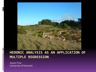
Austin Troy University of Vermont HEDONIC ANALYSIS AS AN APPLICATION OF MULTIPLE REGRESSION
Valuing bundled goods • Being from France is not directly priced, but by comparing price of French and non-French wines can isolate that “premium.” • The value of a 95+ mph split finger fastball (SFF) is not directly priced, but by comparing the contract trading price of a good SFF pitcher against one without, we can begin to price it • Except….
Except… • What if those two pitchers are not otherwise identical? (ie the pitcher without the SFF happens to have several great breaking pitches (e.g. slider), he’s a better batter, a little older, and his ERA is a little lower • Now, in order to see how the SFF affects the contract price, we have to adjust for those other factors—hold them constant. • To make that comparison means we need enough pitchers to analyze such that we have sufficient variation across all those factors (a lot of other assumptions must be fulfilled, but we’ll get into that later)
Now imagine a formula • Price = function of: • SFF (yes/no), • speed of SFF, • binary vector of other types of pitches (yes/no), • vector of average speeds for those pitches • Other stats (ERA, walks, strikes, age, etc.) • If I get an equation that relates 1-5 against Price with sufficient variability in the data set across attributes, I can then “control” for 3-5, and get an estimate of how 1 and 2 contribute to price. • That is, I “unbundled” the price of a major league pitcher to price something that is not directly price in the market
Think of some other “bundled goods” Went a little crazy with the clip art • Cars • Food • Computers • Cell phones • Hotel rooms • Vacation packages • REAL ESTATE
The housing bundle • This “price unbundling” most commonly is applied to real estate because • It’s technically feasible: • There are lots of housing transactions • There are many easily quantifiable attributes • There’s wide variation in housing attributes • It’s important • It’s the single most important asset class; is it being valued correctly? • Housing prices reflect so many non-market goods so it’s a great way to value amenities and disamenities
Some parts of the housing bundle that can be valued: • # bedrooms/bathrooms • Square footage • Attached garage • Age of house • Building material • Luxuries: pool, hot tub, 100 ft tall lawn gnome • Property taxes • Size of lot Proxy for value of raw land • However land value component can be further broken down because it derives from location and…
…can also value things related to location: • “Quality” of neighborhood • You’re buying piece of the neighborhood • Often use proxies like income, crime, tenure, etc. • Municipal services • E.g. school district quality, availability of sewer/water/trash service, etc. • Site factors • Soil/slope constraints, views, climate, easements, hazards • Proximity and accessibility to: • Employment and services • Transportation (transit, highways, etc.) • Amenities and disamenities
Hedonic analysis • Each component yields an “implicit” price, reflective of WTP for a marginal change in a given attribute • Price= fn(structure, neighborhood, location) • The result is a “schedule” of marginal prices for all the elements of home value • Can be used to create housing price indices
Linearity • How does the relationship between price and attributes vary with magnitude of x and y? • One option is to transform independent variables. Here we log transform # rooms • So change in price now depends on number of rooms at which price is evaluated
Functional form: dependent variable transformation • Linear model: 1 unit change in attribute results in change in price; however, linear model is unrealistic • Semi-log model; take ln of price: interpret coefficients as % changes in y due to 1 unit increase in x; ie. Price effect depends on house price level at which evaluated • Log-log model: take ln of both sides: interpret coefficients as elasticities; % change in y due to % change in x; i.e. price effect depend both on level of y and of x variables • Box-Cox model: flexible functional form • Uses a power transformation • Ln, linear and sqrt are “special cases”
Hedonic assumptions: • Single housing market: • All variability in housing prices accounted for • no omitted variable bias. • Proper functional form • No transaction costs • Unlimited “repackaging” of attributes • Independence of observations • Exogeneity • Price is dependent
Sample hedonic studies of open space and forests • Tyrvainen (1997): urban forests in Joensuu, Finland—positive • Lutzenhizer and Netusil (2001) and Bolitzer and Netusil (2000): urban parks in Portland, OR—positive • Netusil (2005): urban parks in Portland OR—positive when the park is more than 200 feet from the property • Thompson, Hanna et al (2004): urban interface tree health and density in Tahoe Basin—positive • Nicholls and Crompton (2005): linear greenways in Austin, TX—positive effect when adjacent
Sample hedonic studies of open space and forests • Acharya and Bennett(2001): % of open space up to 1 mile from a house in CT—positive • Des Rosier (2002): proportion of trees on property relative to surroundings in Quebec City—positive (scarcity effect) • Correllet al.(1978): greenbelts in Boulder, CO—positive • Morancho (2003): park proximity in Castellon; modest increase • Lacy (1990): open space in subdivisions in MA—positive • Espey and Owusu-Edusei (2001): urban parks in Greenville, SC—negative
Example #1 A. Troy and J.M. Grove. 2008. Property Values, parks, and crime: a hedonic analysis in Baltimore, MD. Landscape and Urban Planning. 87:233-245.
Methods • Regress property price for ~25,000 property sales in Baltimore against a range of control variables plus amenity and crime variables • 4 models: 1) ln (d2 park); 2) lin (d2 park); 3) Box Cox trans of price; 4) SAR model, ln(d2 park) = vector of untransformed control variables = vector of control variables to be log-transformed = distance to park = robbery rate for park area =interaction term for previous two =coefficient
Variables • Models: • Log-log • Log-linear • Box-Cox • Spatial MAIN EFFECTS: • 1999 and 2005 robbery rates • Ln distance to nearest park (model 1); distance to nearest park (model 2) CONTROL VARIABLES: • Ln square footage of structure • Ln parcel area • Ln improvement value (assessed) • Bathrooms • Years old • Structure quality • Single family home (1/0) • Year transacted • Whether house is renter occupied (1/0) • Ln median HH income of BG • % HS graduates in BG • % owner occupied in BG • Median age of BG • Ln distance downtown • Distance interstate
Defining and attributing parks • “Parks” under 2 ha and with less than 50% vegetated surface were removed to get rid of things like highway buffers, median strips, paved pocket parks and other park “fragments” with low amenity value
Results R-squared of .66 Relatively low fit relates to problems with central city property data All control variables significant with expected sign Main effects are expected sign and significance Interaction is significant Almost no difference when using 1999 vs 2005 crime data
Results: park & crime interaction • For lower crime levels, price increases with proximity to park, all else constant. • As crime rate increases, curve gets less steep • At a certain crime level, (~450% of national average) the curve reverses direction • Mean 2005 robbery index is 475% of national average for Baltimore
Results: tree percentage • Above ~450% crime levels, property price decreases with proximity to parks • Gets steeper as crime rate increases • At mean crime rate for city (475%), parks are valued negatively!
Model 2: linear versions Result basically the same, but get lines instead of asymptotic curves