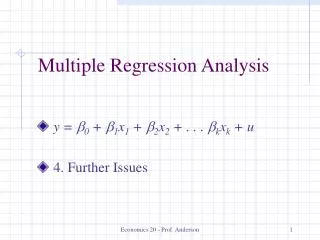
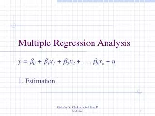
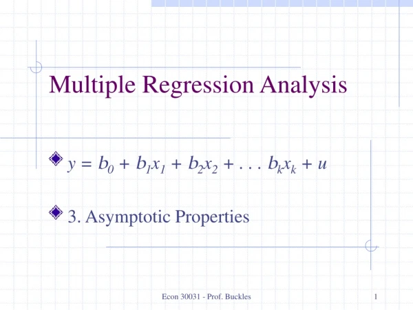
Multiple Regression Analysis
Multiple Regression Analysis. Week 12 GT00303. Multiple Regression. In Week 11, we covered Simple Regression Model which analyzes the relationship between the dependent variable (y) and another ONE independent variable (x).

Multiple Regression Analysis
E N D
Presentation Transcript
Multiple Regression Analysis Week 12 GT00303
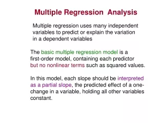
Multiple Regression In Week 11, we covered Simple Regression Model which analyzes the relationship between the dependent variable (y) and another ONE independent variable (x). Multiple Regression Model allows for any number of independent variables. Since the manual computation is time-consuming, our analysis will be performed using Excel. The focus hence will be on the interpretation of output. 12-2
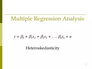
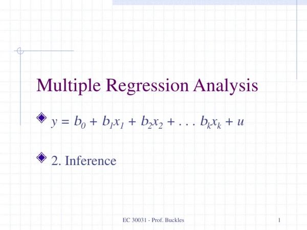
Multiple Linear Regression Model Population Sample For x =1, we drew a regression line For x > 1, we imagine a response surface. 12-4
Required Conditions As before, the Multiple Regression Model is valid only if the following four conditions for the error variable (ε) are met: 1) The probability distribution of ε is normal. 2) The mean of ε is 0. 3) The standard deviation of εis constant. 4) εare independent. These conditions can be checked by performing Residual Analysis. 12-5
Steps in Regression Analysis 1. Develop a model that has a theoretical basis and collect data for all variables. 2. Use software to perform the regression analysis and generate the output. 3. Perform residuals diagnostic to check for violations of required conditions. If there are problems, attempt to remedy them. 4. Assess the model’s fit(using standard error of estimate, R2, and ANOVA) 5. If the model fits the data, use the regression equation to predict a particular value of the dependent variable and/or estimate its mean. 12-6
Case Study: Determinants of Income Using data from General Social Survey, we would like to identify the variables that affect one’s income. Here is a list of variables that may be linearly related to income. 12-7
Step 1: 12-8
Step 2: 12-9
Step 3: 12-12
Step 4: We will assess the model in three ways: Standard error of estimate (sε) Coefficient of determination (R2) F-test of the analysis of variance (ANOVA) 12-13
When all the sample data points are on the regression line (perfect fit), SSE = 0, and hence sε = 0. • If sε is small, the fit is excellent, and the linear model should be used for forecasting. • If sε is large, the model is a poor one. It appears that the standard error of estimate (33250) is quite large! 12-15
Coefficient of Determination (R2) The statistic tells us that 33.74% of the variation in income is explained by the variation in the 8 independent variables. The remaining 66.26% is unexplained by the model (due to other factors captured by the error term). 12-16
If k is large relative to n, the R2 may be unrealistically high. The adjusted R2 (coefficient of determination adjusted for degrees of freedom) takes into account n and k. If n is considerably larger than k, R2 ≈ Adjusted R2 12-17
ANOVA • H0: β1 = β2 = … = βk = 0 • H1: At least one βi is not equal to zero If H0 is true (Do not reject H0), none of the independent variables is linearly related to y. • The model is invalid. If H0is false (Reject H0), at least one of the independent variables is linearly related to y. • The model does have some validity. 12-18
If F is large, most of the variation in y is explained by the regression equation. • The model is valid. If Fis small, most of the variation in y is unexplained by the regression equation. • The model is invalid. 12-19
Is the value of F large? This is a one-tail (right tail) test. 12-20
p-value = 7.02 x 10⁻²¹ ≈ 0.0000 • Reject H0 and conclude there is overwhelming evidence at least one of the independent variables is linearly related to y, and hence the model is valid. 12-21
Step 5: Once we aresatisfied that the model fits the data as well as possible, and that the required conditions are satisfied, we can interpret and test the individual coefficients and use the model to predict and estimate. 12-22
Statistical Significance of Coefficients H0: βi = 0 H1: βi≠ 0 12-26
The results show that there is no evidence of a linear relationship for CHILDS, EARNRS, CUREMPYR. However, it may also mean that there is a linear relationship between the two variables, but the problem of multicollinearity distorts the t-test and reveals no linear relationship. 12-28
Predicting Using the Regression To illustrate, we will predict the income of a 50-year old, with 12 years of education, who works 40 hours per week, whose spouse also works 40 hours per week, has an occupation prestige score of 50, has 2 children, 2 earners in the family, and has worked for the same company for 5 years. 12-29
Do note that it is unreliable to extrapolate far outside the range of the observed values of the independent variables. 12-30
Multicollinearity Multiple regression models have a problem that simple regressions do not, namely multicollinearity. It happens when the independent variables are highly correlated. Multicollinearity distorts the t-tests of the coefficients, making it difficult to determine the existence of a linear relationship. Fortunately, it does not affect the F-test of the analysis of variance. 12-31
For instance, a simple correlation test shows that there is a significant linear relationship between: • INCOME and AGE • INCOME and CUREMPYR BUT the multiple regression shows otherwise! How to reconcile the contradicting results?? 12-32
Multicollinearity affects the results of the multiple regression t-tests so that it appears that both AGE and CUREMPYR are not statistically significant when in fact both variables are linearly related to INCOME. This is because AGE and CUREMPYR are highly correlated! 12-34
How to deal with multicollinearity? Minimizing the effect of multicollinearity is often easier than correcting it. The statistics practitioner must try to include independent variables that are independent of each other. Another alternative is to use a stepwise regression package. 12-35

