Download
1 / 32
320 likes | 421 Views
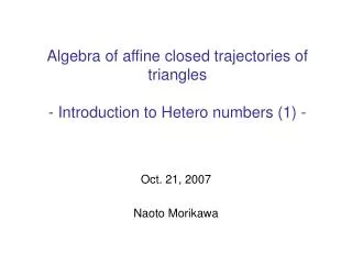
Algebra of affine closed trajectories of triangles - Introduction to Hetero numbers (1) -. Oct. 21, 2007 Naoto Morikawa. Outline of the talk. Introduction and motivation Lattices, cones, and roofs Surface decomposition by conjugate roof Algebra of roofs and hetero numbers.

E N D
Algebra of affine closed trajectories of triangles- Introduction to Hetero numbers (1) - Oct. 21, 2007 Naoto Morikawa
Outline of the talk • Introduction and motivation • Lattices, cones, and roofs • Surface decomposition by conjugate roof • Algebra of roofs and hetero numbers
Flow of triangles Division on 3-cube “Peaks & valleys” Flow of triangles Divide facets of 3-cube [0,1]3into triangles Pile up the 3-cubes along the direction of (-1, -1, -1) Project the surface on a hyperplane that is (-1, -1, -1) (-∞, -∞, -∞) (0,0,0) (0,0,1) (1,0,0) trajectory (0,1,0) (+∞, +∞, +∞)
Example: affine closed trajectory • “Peaks and valleys” defined by three peaks, (l, m, n), (l+1, m-1, n), and (l+2, m+1, n-1) Z3, specifies a closed trajectory of length 10. (l+1, m-1, n) (l, m, n) (l+2, m+1, n-1) Closed trajectory (1, 0, 0) (0, 0, 1) (0, 1, 0) [NOTE] Affine closed trajectory := closed trajectory specified by a single set of “peaks and valleys”
Motivation of the talk • One could specify any affine closed trajectory by “peaks and valleys” of the ”conjugate” lattice. • As a result, we could describe “fusion and fission” of closed trajectories as addition of the corresponding “conj. peaks & valleys” “Peaks & valleys” of conj. lattice “Standard” lattice which is generated by (1, 0, 0), (0, 1, 0), (0, 0, 1) “Conjugate” lattice which is generated by (0, 1, 1), (1, 0, 1), (1, 1, 0)
Notation: monomial representation • We denote point (l, m, n)R3 by monomial x1lx2mx3n of three indeterminates x1, x2, and x3: (l+1, m-1, n) x1l+1x2m-1x3n (l, m, n) x1lx2mx3n (l+2, m+1, n-1) x1l+2x2m+1x3n-1 (0, 0, 1) x3 (1, 0, 0) x1 x2 (0, 1, 0)
Outline of the talk • Introduction and motivation • Lattices, cones, and roofs • Surface decomposition by conjugate roof • Algebra of roofs and hetero numbers
Standard lattice • [Def’n] The standard lattice L3 is the lattice which is generated by x1, x2, and x3 • The standard lattice L3 is used to specify a flow of triangles “Peaks & valleys” of conj. lattice “Standard” lattice which is generated by x1 i.e. (1, 0, 0), x2 i.e. (0, 1, 0), x3 i.e. (0, 0, 1) “Conjugate” lattice which is generated by (0, 1, 1), (1, 0, 1), (1, 1, 0)
x3 x1 x2 Standard cone (“tangent” cone) • [Def’n] For A = { x1lix2mix3ni } L3, Cone A := { (l, m, n) R3 : l li, m mi, n ni for some x1lix2mix3ni A } • Cone A specifies “peaks and valleys” of the standard lattice generated by A x1l+1x2m-1x3n x1lx2mx3n x1l+2x2m+1x3n-1 “Standard” lattice which is generated by x1 = (1, 0, 0), x2 = (0, 1, 0), x3 = (0, 0, 1) “Conjugate” lattice which is generated by (0, 1, 1), (1, 0, 1), (1, 1, 0) Cone { x1lx2mx3n, x1l+1x2m-1x3n, x1l+2x2m+1x3n-1 }
Conjugate lattice • [Def’n] The conjugate lattice L3 is the lattice which is generated by x2x3, x1x3, and x1x2 • The conjugate lattice L3 is used to specify the “boundary” of a trajectory x3 x1 y2 y1 x2 y3 “Conjugate” lattice which is generated by y1 := x2x3 i.e. (0, 1, 1), y2 := x1x3 i.e. (1, 0, 1), y3 := x1x2 i.e. (1, 1, 0) Note that the conjugate lattice is “sparse”: “Standard” lattice which is generated by x1 = (1, 0, 0), x2 = (0, 1, 0), x3 = (0, 0, 1) L3 L3 + xiL3
y2 y1 y3 Conjugate cone (“cotangent” cone) • [Def’n] For A = { x1lix2mix3ni } L3, Cone A := { (l, m, n) R3 : -l+m+n -li+mi+ni, l-m+n li-mi+ni, l+m-n li+mi-ni, for some x1lix2mix3ni A } Note that x1lx2mx3n = y1(-l+m+n)/2y2(l-m+n)/2y3(l+m-n)/2. • Cone A specifies “peaks and valleys” of the conjugate lattice generated by A x1l+1x2m-1x3n x1lx2mx3n x1l+2x2m+1x3n-1 “Conjugate” lattice which is generated by x2x3 = (0, 1, 1), x1x3 = (1, 0, 1), x1x2 = (1, 1, 0) “Standard” lattice which is generated by x1 = (1, 0, 0), x2 = (0, 1, 0), x3 = (0, 0, 1) Cone { x1lx2mx3n, x1l+1x2m-1x3n, x1l+2x2m+1x3n-1 }
y2 y1 y3 Conjugate roof • [Def’n] For A L3, Roof A := { (m+n, l+n, l+m) R3 : y1l+Ny2my3n, y1ly2m+Ny3n, y1ly2my3n+N Cone A for some N > 0} Note that x1m+nx2l+nx3l+m = y1ly2my3n. • Roof A is obtained by putting as many cubes as possible on Cone A x1l-1x2m-1x3n-1 “Conjugate” lattice which is generated by x2x3 = (0, 1, 1), x1x3 = (1, 0, 1), x1x2 = (1, 1, 0) “Standard” lattice which is generated by x1 = (1, 0, 0), x2 = (0, 1, 0), x3 = (0, 0, 1) Roof { x1lx2mx3n, x1l+1x2m-1x3n, x1l+2x2m+1x3n-1 } ( = Cone { x1l-1x2m-1x3n-1 } )
y2 y1 y3 Extended conjugate cone • [Def’n] For A L3, XCone A := Cone A Cone x1A Cone x2A Cone x3A, where xiA = { xia | a A } • Since the conjugate lattice L3 is “sparse” (L3 L3 + xiL3), one should use extended cones to capture all the “boundary” of trajectories x1l+1x2m-1x3n x1lx2mx3n x1l+2x2m+1x3n-1 “Conjugate” lattice which is generated by x2x3 = (0, 1, 1), x1x3 = (1, 0, 1), x1x2 = (1, 1, 0) “Standard” lattice which is generated by x1 = (1, 0, 0), x2 = (0, 1, 0), x3 = (0, 0, 1) XCone { x1lx2mx3n, x1l+1x2m-1x3n, x1l+2x2m+1x3n-1 }
y2 y1 y3 Extended conjugate roof • [Def’n] For A L3, XRoof A := the conjugate roof of XCone A • XRoof A is obtained by putting as many cubes as possible on XCone A x1l-1x2m-1x3n-1 x1lx2m-1x3n x1l+1x2m-1x3n-1 “Conjugate” lattice which is generated by x2x3 = (0, 1, 1), x1x3 = (1, 0, 1), x1x2 = (1, 1, 0) “Standard” lattice which is generated by x1 = (1, 0, 0), x2 = (0, 1, 0), x3 = (0, 0, 1) x1lx2mx3n-1 XRoof { x1lx2mx3n, x1l+1x2m-1x3n, x1l+2x2m+1x3n-1 } ( = XCone { x1l-1x2m-1x3n-1, x1l+1x2m-1x3n-1, x1lx2mx3n-1 , x1lx2m-1x3n } )
Summary of lattices, cones, and roofs • Cone A is defined to specify the “gradient” of triangles. ==> Cone A is used to specify a flow of tetrahedrons • Roof A is defined to specify the “boundary” of a trajectory ==> Roof A (or XRoof A) is used to specify a trajectory Cone {p1, p2, p3} Roof {p1, p2, p3} XRoof {p1, p2, p3} p1 p3 p2
Outline of the talk • Introduction and motivation • Lattices, cones, and roofs • Surface decomposition by conjugate roof • Algebra of roofs and hetero numbers
x3 x1 x2 Notation : triangles on Cone A • We denote the triangle of vertices a (=x1lx2mx3n), axi, axixj by a[xixj] • We denote the projection of a[xixj] on the hyperplane by |a[xixj]| “Slant” triangles Cone A (A L3) a a ax1 ax2 “Flat” triangles ax1x2 ax1x2 (a) (a) (ax1) a[x2x1] a[x1x2] (ax2) (ax1x2) (ax1x2) |a[x2x1]| |a[x1x2]|
Surface decomposition by Roof A • Slant triangles on Cone A (A L3) are classified into three kinds: - In(Cone A, Roof A) := the slant triangles under Roof A - Bd(Cone A, Roof A) := the slnt tri. partially covered by Roof A - Out(Cone A, Roof A) := the slant triangles above Roof A “In” Cone A & Roof A “Out”
Surface decomposition (cont’d) • Slant triangles on Cone A (A L3)are classified into three kinds: - In(Cone A, Roof A) := the slant triangles under Roof A - Bd(Cone A, Roof A) := the slnt tri. partially covered by Roof A - Out(Cone A, Roof A) := the slant triangles above Roof A • We denote the projection on the hyperplane by In(A): In(A) := { |a[xixj]| | a[xixj] In(Cone A, Roof A) } All vertices are on orunder the surface of Roof A “In” Above Roof A Surface of Roof A In(A) Under Roof A
Surface decomposition (cont’d) • Slant triangles on Cone A (A L3)are classified into three kinds: - In(Cone A, Roof A) := the slant triangles under Roof A - Bd(Cone A, Roof A) := the slnt tri. partially covered by Roof A - Out(Cone A, Roof A) := the slant triangles above Roof A Top vertex is above and bottom vertex is under the surface of Roof A “Boundary” Above Roof A Bd(Cone A, Roof A) = in the above example Surface of Roof A Under Roof A
Surface decomposition (cont’d) • Slant triangles on Cone A (A L3)are classified into three kinds: - In(Cone A, Roof A) := the slant triangles under Roof A - Bd(Cone A, Roof A) := the slnt tri. partially covered by Roof A - Out(Cone A, Roof A) := the slant triangles above Roof A All vertices are on orabove the surface of Roof A “Out” Above Roof A Surface of Roof A Under Roof A
Surface decomposition (summary) • Slant triangles on Cone A (A L3) are classified into three kinds: - In(Cone A, Roof A) := the slant triangles under Roof A - Bd(Cone A, Roof A) := the slnt tri. partially covered by Roof A - Out(Cone A, Roof A) := the slant triangles above Roof A In Bd Out Another example
Decomposition & Trajectory • Given A L3. If Bd(Cone A, Roof A)= , then no trajectory defined by Cone A crosses the boundary of “In” and “Out”. In particular, - In(Cone A, Roof A) <=> all the closed trajectories - Out(Cone A, Roof A) <=> all the open trajectories Bd = Bd Bd =
Decomposition & Trajectory (cont’d) • Extended conjugate roof XRoof A gives a “larger neighborhood”: - In(Cone A, XRoof A) includes all the closed trajectories - Usually, Bd(Cone A, XRoof A) • XRoof A is mainly used in the 3-dim’l case to capture all the closed trajectories which visit at least one of the peaks of Cone A Bd Bd Bd
Outline of the talk • Introduction and motivation • Lattices, cones, and roofs • Surface decomposition by conjugate roof • Algebra of roofs and hetero numbers
x3 x1 x2 Standard roof • [Def’n] For A L3, Roof A := { (l, m, n) R3 : (l + N, m, n), (l, m + N, n), (l, m, n + N) Cone A for some N > 0} • Roof A is obtained by putting as many cubes as possible on Cone A Cone A Roof A x1lx2mx3n x1lx2mx3n+1 x1l+1x2mx3n x1lx2m+2x3n Roof { x1l+1x2mx3n, x1lx2m+2x3n, x1lx2mx3n+1 } ( = Cone { x1lx2mx3n } )
Addition of roofs • [Def’n] For A and B L3, Roof A + Roof B := Roof AB • In general, InR(A) InR(B) InR(AB), where InR(X) := { |a[xixj]| | a[xixj] In(Roof X, Roof X) } Roof A + Roof B Roof A +Roof B +Roof C Roof A +Roof B +Roof D InR(A) InR(A) InR(A) InR(AB) InR(C) InR(ABC) InR(D) InR(DAB) InR(B) InR(B) InR(B) Recall that In(X) := { |a[xixj]| | a[xixj] In(Cone X, Roof X) }.
Equivalence relation on cones • [Def’n] For A and B L3, we introduce an equiv. relation on cones: where g(X) denotes the peaks of Cone X. The equivalence class of Cone A is denoted by [Cone A]R • Then, In(A) = In(B) if [Cone A]R = [Cone B]R Roof A = Roof B, Roof g(A) = Roof g(B) Cone A Cone B <=> Cone A Cone A{x1x2x3-2} Cone A{x2 ,x1x2x3-2} where A ={ x1, x3, x1x22x3-2, x1-1x2x3, x1-1x23}
Addition of [Cone A]R • [Def’n] For A and B L3, [Cone A]R + [Cone B]R := [Cone AB]R • If g(A)g(B) = g(C), then [Cone A]R + [Cone B]R = [Cone C]R <=> Roof A + Roof B = Roof C, Roof g(A) + Roof g(B) = Roof g(C) [Cone A]R + [Cone B]R + [Cone C]R + [Cone D]R [Cone A]R + [Cone E]R [Cone F]R + [Cone D]R = = In(E) In(D) In(D) In(B) In(C) In(A) In(A) In(F)
Hetero Numbers • [Def’n] Hetero numbers HNare defined as follows: HN := { [Cone A]R : A L3, Bd(Cone A, Roof A) = }, [Cone A]R + [Cone B]R := [Cone AB]R • Recall that, if Bd(Cone A, Roof A) = , then In(Cone A, Roof A) <=> all the closed trajectories Bd = Bd Bd =
Example: “fusion & fission” of closed traj.s • For [Cone A]R HN, the equiv. class gives all the “partitions” of In(A) into closed trajectories • In particular, we could describe “fusion and fission” of closed trajectories as “addition” of the corresponding hetero numbers Cone G [Cone G]R In(E) [Cone G]R = [Cone A]R + [Cone E]R In(A) In(G) = In(A)In(E) [Cone G]R = [Cone A]R + [Cone B]R + [Cone C]R + [Cone D]R In(B) In(C) In(G) = In(A)In(B)In(C)In(D) In(G) In(D) [Cone G]R = [Cone F]R + [Cone D]R In(G) = In(F)In(D) In(F) A = {x22, x1x3-1, x1x2x3-2}, B = {x2x3, x1x2-1, x1x3-1}, C = {x22, x2x3, x1-1x22x3}, D = {x32, x2x3, x1-1x2x32}, E = {x22, x32, x1x3-1, x1x2-1, x1-1x22x3, x1-1x2x32}, F = {x2, x1x3-1, x1x2-1, x1x2x3-2, x1-1x22x3}, G = ABCD
Example: “fusion & fission” of closed traj.s • For [Cone A]R HN, the equiv. class gives all the “partitions” of In(A) into closed trajectories • In particular, we could describe “fusion and fission” of closed trajectories as “addition” of the corresponding hetero numbers Cone G Thank you! [Cone G]R In(E) [Cone G]R = [Cone A]R + [Cone E]R In(A) In(G) = In(A)In(E) [Cone G]R = [Cone A]R + [Cone B]R + [Cone C]R + [Cone D]R In(B) In(C) In(G) = In(A)In(B)In(C)In(D) In(G) In(D) [Cone G]R = [Cone F]R + [Cone D]R In(G) = In(F)In(D) In(F) A = {x22, x1x3-1, x1x2x3-2}, B = {x2x3, x1x2-1, x1x3-1}, C = {x22, x2x3, x1-1x22x3}, D = {x32, x2x3, x1-1x2x32}, E = {x22, x32, x1x3-1, x1x2-1, x1-1x22x3, x1-1x2x32}, F = {x2, x1x3-1, x1x2-1, x1x2x3-2, x1-1x22x3}, G = ABCD